Concentration is often given in grams per litre (g L−1) rather than kilograms per cubic metre (kg m−3).
Note also that 1 mg mL−1 is therefore also equal to 1 kg m−3.
Molarity is commonly expressed as mol L−1 and often written using the symbol M or m; its conversion to SI units is
2.1.1 Weight or volume concentration
Concentration is often expressed as the weight of solute in a unit volume of solution; for example, g dm−3, or as % w/v, which is the number of grams of solute in 100 mL of solution. When the solute is a liquid, the concentration may also be expressed as the volume of solute in a unit volume of solution, for example as % v/v, which is the number of mL of solute in 100 mL of solution. These are not exact methods when working at a range of temperatures, since the volume of the solution is temperature dependent and hence the weight or volume concentrations also change with temperature.
Whenever a hydrated compound is used it is important to use the correct state of hydration in the calculation of weight concentration. Thus, 10% w/v CaCl2 (anhydrous) is approximately equivalent to 20% w/v CaCl2·6H2O and consequently the use of the vague statement ‘10% calcium chloride’ could result in gross error.
When very dilute solutions are involved the concentration may be expressed as parts per million (or ppm), which is the number of grams in 106 grams of solution (which equals the number of mg per kg of solution) or, if the solute is a liquid, the number of mL in 106 mL (1000 litres) of solution. Since the density of very dilute aqueous solutions at room temperature approximates to 1 g mL−1, a concentration of 1 ppm is approximately 1 mg of solute per litre of solution (i.e. 1 g in 106 mL).
2.1.2 Molarity and molality
These two similar-sounding terms should not be confused. The molarity of a solution is the number of moles (gram molecular weights) of solute in 1 litre (1 dm3) of solution. The molality is the number of moles of solute in 1 kg of solvent. Molality has the unit, mol kg−1, which is an accepted SI unit. Molarity may be converted to SI units as shown in Box 2.1; interconversion between molarity and molality requires knowledge of the density of the solution.
Of the two units, molality is preferable for a precise expression of concentration because, unlike molarity, it does not depend on the solution temperature; also, the molality of a component in a solution remains unaltered by the addition of a second solute, whereas the molarity of the first component decreases because the total volume of solution increases following the addition of the second solute.
2.1.3 Milliequivalents
These units are commonly used clinically in expressing the concentration of an ion in solution. The term ‘equivalent’ or ‘gram equivalent weight’ is analogous to the mole or gram molecular weight. When monovalent ions are considered, these two terms are identical. A 1 molar (1 mol L−1) solution of sodium bicarbonate (sodium hydrogen carbonate), NaHCO3, contains 1 mol or 1 Eq of Na+ and 1 mol or 1 Eq of HCO3− per litre of solution. With multivalent ions, attention must be paid to the valency of each ion; for example, 10% w/v CaCl2·2H2O contains 6.8 mmol or 13.6 mEq of Ca2+ in 10 cm3.
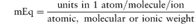
The Pharmaceutical Codex1 gives a table of milliequivalents for various ions and also a simple formula for the calculation of milliequivalents per litre (Box 2.2).
Box 2.2 Calculation of milliequivalents |
The number of milliequivalents in 1 g of substance is given by
For example, CaCl2·2H2O (mol wt = 147.0 Da):
and
that is, each gram of CaCl2·2H2O represents 13.6 mEq of calcium and 13.6 mEq of chloride. |


In analytical chemistry, a solution that contains 1 Eq per litre is referred to as a normal solution. Unfortunately the term ‘normal’ is also used to mean physiologically normal with reference to saline solution. In this usage, a physiologically normal saline solution contains 0.9 g NaCl in 100 cm3 aqueous solution and not 1 equivalent (58.44 g) per litre.
2.1.4 Mole fraction
The mole fraction of a component of a solution is the number of moles of that component divided by the total number of moles present in solution. In a two-component (binary) solution, the mole fraction of solvent, x1, is given by x1 = n1/(n1 + n2), where n1 and n2 are, respectively, the number of moles of solvent and solute present in solution. Similarly, the mole fraction of solute, x2, is given by x2 = n2/(n1 + n2). The sum of the mole fractions of all components is, of course, unity, i.e. for a binary solution, x1 + x2 = 1.
|
Isotonic saline contains 0.9% w/v of sodium chloride (mol wt = 58.5 Da). Express the concentration of this solution as: (a) molarity; (b) molality; (c) mole fraction; and (d) milliequivalents of Na+ per litre. Assume that the density of isotonic saline is 1 g cm−3. Answer (a) 0.9% w/v solution of sodium chloride contains 9 g dm−3 = 0.154 mol dm−3. (b) 9 g of sodium chloride is dissolved in 991 g of water (assuming density = 1 g cm−3). Therefore, 1000 g of water contains 9.08 g of sodium chloride = 0.155 mol, i.e. molality = 0.155 mol kg−1. (c) Mole fraction of sodium chloride, x1, is given by
(Note: 991 g of water contains 991/18 moles, i.e. n2 = 55.06.) (d) Since Na+ is monovalent, the number of milliequivalents of Na+ = number of millimoles. Therefore, the solution contains 154 mEq dm−3 of Na+. |

2.2 Thermodynamics: a brief introduction
The importance of thermodynamics in the pharmaceutical sciences is apparent when it is realised that such processes as the partitioning of solutes between immiscible solvents, the solubility of drugs, micellisation and drug–receptor interaction can all be treated in thermodynamic terms. This brief section merely introduces some of the concepts of thermodynamics that are referred to throughout the book. Readers requiring a greater depth of treatment should consult standard texts on this subject.2
2.2.1 Energy
Energy is a fundamental property of a system. Some idea of its importance may be gained by considering its role in chemical reactions, where it determines what reactions may occur, how fast the reaction may proceed, and in which direction the reaction will occur. Energy takes several forms: kinetic energy is that which a body possesses as a result of its motion; potential energy is the energy a body has due to its position, whether gravitational potential energy or coulombic potential energy associated with charged particles at a given distance apart. All forms of energy are related, but in converting between the various types it is not possible to create or destroy energy. This forms the basis of the law of conservation of energy.
The internal energy U of a system is the sum of all the kinetic and potential energy contributions to the energy of all the atoms, ions and molecules in that system. In thermodynamics we are concerned with change in internal energy, ΔU, rather than the internal energy itself. (Notice the use of Δ to denote a finite change.) We may change the internal energy of a closed system (one that cannot exchange matter with its surroundings) in only two ways: by transferring energy as work (w) or as heat (q). An expression for the change in internal energy is

If the system releases its energy to the surroundings, ΔU is negative, i.e. the total internal energy has been reduced. Where heat is absorbed (as in an endothermic process), the internal energy will increase and consequently q is positive. Conversely, in a process that releases heat (an exothermic process) the internal energy is decreased and q is negative. Similarly, when energy is supplied to the system as work, w is positive and when the system loses energy by doing work, w is negative.
It is frequently necessary to consider infinitesimally small changes in a property; we denote these by the use of d rather than Δ. Thus, for an infinitesimal change in internal energy we write equation (2.1) as

We can see from this equation that it does not really matter whether energy is supplied as heat or as work or as a mixture of the two: the change in internal energy is the same. Equation (2.2) thus expresses the principle of the law of conservation of energy but is much wider in its application since it involves changes in heat energy, which were not encompassed in the conservation law.
It follows from equation (2.2) that a system that is completely isolated from its surroundings, such that it cannot exchange heat or interact mechanically to do work, cannot experience any change in its internal energy. In other words, the internal energy of an isolated system is constant – this is the first law of thermodynamics.
2.2.2 Enthalpy
When a change occurs in a system at constant pressure as, for example, in a chemical reaction in an open vessel, the increase in internal energy is not equal to the energy supplied as heat because some energy will have been lost by the work done (against the atmosphere) during the expansion of the system. It is convenient, therefore, to consider the heat change in isolation from the accompanying changes in work. For this reason we consider a property that is equal to the heat supplied at constant pressure: this property is called the enthalpy (H). We can define enthalpy by

ΔH is positive when heat is supplied to a system that is free to change its volume and negative when the system releases heat (as in an exothermic reaction). Enthalpy is related to the internal energy of a system by the relationship

where p and V are the pressure and volume of the system, respectively.
Enthalpy changes accompany such processes as the dissolution of a solute, the formation of micelles, chemical reaction, adsorption on to solids, vaporisation of a solvent, hydration of a solute, neutralisation of acids and bases, and the melting or freezing of solutes.
2.2.3 Entropy
The first law, as we have seen, deals with the conservation of energy as the system changes from one state to another, but it does not specify which particular changes will occur spontaneously. The reason why some changes have a natural tendency to occur is not that the system is moving to a lower-energy state but that there are changes in the randomness of the system. This can be seen by considering a specific example: the diffusion of one gas into another occurs without any external intervention – i.e. it is spontaneous – and yet there are no differences in either the potential or kinetic energies of the system in its equilibrium state and in its initial state where the two gases are segregated. The driving force for such spontaneous processes is the tendency for an increase in the chaos of the system – the mixed system is more disordered than the original.
A convenient measure of the randomness or disorder of a system is the entropy (S). When a system becomes more chaotic, its entropy increases in line with the degree of increase in disorder caused. This concept is encapsulated in the second law of thermodynamics, which states that the entropy of an isolated system increases in a spontaneous change.
The second law, then, involves entropy change, ΔS, and this is defined as the heat absorbed in a reversible process, qrev, divided by the temperature (in kelvins) at which the change occurred.
For a finite change,

and for an infinitesimal change,

By a ‘reversible process’ we mean one in which the changes are carried out infinitesimally slowly, so that the system is in equilibrium with its surroundings. In this case we infer that the temperature of the surroundings is infinitesimally higher than that of the system and consequently the heat changes are occurring at an infinitely slow rate, so that the heat transfer is smooth and uniform.
We can see the link between entropy and disorder by considering some specific examples. For instance, the entropy of a perfect gas changes with its volume V according to the relationship
where the subscripts f and i denote the final and initial states. Note that if Vf > Vi (i.e. if the gas expands into a larger volume) the logarithmic (ln) term will be positive and the equation predicts an increase of entropy. This is expected since expansion of a gas is a spontaneous process and will be accompanied by an increase in the disorder because the molecules are now moving in a greater volume.
Similarly, increasing the temperature of a system should increase the entropy because at higher temperature the molecular motion is more vigorous and hence the system is more chaotic. The equation that relates entropy change to temperature change is
where CV is the molar heat capacity at constant volume. Inspection of equation (2.8) shows that ΔS will be positive when Tf > Ti, as predicted.
The entropy of a substance will also change when it undergoes a phase transition, since this too leads to a change in the order. For example, when a crystalline solid melts, it changes from an ordered lattice to a more chaotic liquid (Fig. 2.1) and consequently an increase in entropy is expected. The entropy change accompanying the melting of a solid is given by

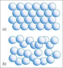
Figure 2.1 Melting of a solid involves a change from an ordered arrangement of molecules, represented by (a), to a more chaotic liquid, represented by (b). As a result, the melting process is accompanied by an increase in entropy.
where ΔHfus is the enthalpy of fusion (melting) and T is the melting temperature. Similarly, we may determine the entropy change when a liquid vaporises from

where ΔHvap is the enthalpy of vaporisation and T now refers to the boiling point. Entropy changes accompanying other phase changes, such as change of the polymorphic form of crystals (see section 1.2.3), may be calculated in a similar manner.
At absolute zero all the thermal motions of the atoms of the lattice of a crystal will have ceased and the solid will have no disorder and hence a zero entropy. This conclusion forms the basis of the third law of thermodynamics, which states that the entropy of a perfectly crystalline material is zero when T = 0.
2.2.4 Free energy
The free energy is derived from the entropy and is, in many ways, a more useful function to use. The free energy referred to when we are discussing processes at constant pressure is the Gibbs free energy (G). This is defined by:

The change in the free energy at constant temperature arises from changes in enthalpy and entropy and is

Thus, at constant temperature and pressure,

from which we can see that the change in free energy is another way of expressing the change in overall entropy of a process occurring at constant temperature and pressure.
In view of this relationship, we can now consider changes in free energy that occur during a spontaneous process. From equation (2.13) we can see that ΔG will decrease during a spontaneous process at constant temperature and pressure. This decrease will occur until the system reaches an equilibrium state when ΔG becomes zero. This process can be thought of as a gradual using up of the system’s ability to perform work as equilibrium is approached. Free energy can therefore be looked at in another way in that it represents the maximum amount of work, wmax (other than the work of expansion) that can be extracted from a system undergoing a change at constant temperature and pressure; i.e.
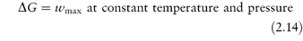
This non-expansion work can be extracted from the system as electrical work, as in the case of a chemical reaction taking place in an electrochemical cell, or the energy can be stored in biological molecules such as adenosine triphosphate.
When the system has attained an equilibrium state, it no longer has the ability to reverse itself. Consequently all spontaneous processes are irreversible. The fact that all spontaneous processes taking place at constant temperature and pressure are accompanied by a negative free-energy change provides a useful criterion of the spontaneity of any given process.
By applying these concepts to chemical equilibria we can derive (see Derivation Box 2A) the following simple relationship between free-energy change and the equilibrium constant of a reversible reaction, K:

where the standard free energy G is the free energy of 1 mole of gas at a pressure of 1 bar.
A similar expression may be derived for reactions in solutions using the activities (see section 2.3.1) of the components rather than the partial pressures. ΔG values can readily be calculated from the tabulated data and hence equation (2.15) is important because it provides a method of calculating the equilibrium constants without resort to experimentation.
A useful expression for the temperature dependence of the equilibrium constant is the van’t Hoff equation, which may be derived as outlined in Derivation Box 2B.
A more general form of this equation is:
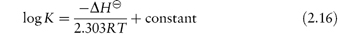
Plots of log K against 1/T should be linear with a slope of −ΔH /2.303R, from which ΔH
 may be calculated.
Equations (2.15) and (2.16) are fundamental equations that find many applications in the broad area of the pharmaceutical sciences: for example, in the determination of equilibrium constants in chemical reactions and for micelle formation; in the treatment of stability data for some solid-dosage forms (see section 3.4.3 in Chapter 3); and for investigations of drug–receptor binding.
|
|

2.3 Activity and chemical potential
2.3.1 Activity and standard states
The term activity is used in the description of the departure of the behaviour of a solution from ideality. In any real solution, interactions occur between the components which reduce the effective concentration of the solution. The activity is a way of describing this effective concentration. In an ideal solution or in a real solution at infinite dilution, there are no interactions between components and the activity equals the concentration. Non-ideality in real solutions at higher concentrations causes a divergence between the values of activity and concentration. The ratio of the activity to the concentration is called the activity coefficient, γ; that is,

Depending on the units used to express concentration we can have a molal activity coefficient, γm, a molar activity coefficient, γc, or, if mole fractions are used, a rational activity coefficient, γx.
In order to be able to express the activity of a particular component numerically, it is necessary to define a reference state in which the activity is arbitrarily unity. The activity of a particular component is then the ratio of its value in a given solution to that in the reference state. For the solvent, the reference state is invariably taken to be the pure liquid, and, if this is at a pressure of 1 atmosphere and at a definite temperature, it is also the standard state. Since the mole fraction as well as the activity is unity: γx = 1.
Several choices are available in defining the standard state of the solute. If the solute is a liquid that is miscible with the solvent (as, for example, in a benzene–toluene mixture) then the standard state is again the pure liquid. Several different standard states have been used for solutions of solutes of limited solubility. In developing a relationship between drug activity and thermodynamic activity, the pure substance has been used as the standard state. The activity of the drug in solution was then taken to be the ratio of its concentration to its saturation solubility. The use of a pure substance as the standard state is of course of limited value since a different state is used for each compound. A more feasible approach is to use the infinitely dilute solution of the compound as the reference state. Since the activity equals the concentration in such solutions, however, it is not equal to unity as it should be for a standard state. This difficulty is overcome by defining the standard state as a hypothetical solution of unit concentration possessing, at the same time, the properties of an infinitely dilute solution. Some workers3 have chosen to define the standard state in terms of an alkane solvent rather than water; one advantage of this solvent is the absence of specific solute–solvent interactions in the reference state that would be highly sensitive to molecular structure.
2.3.2 Activity of ionised drugs
A large proportion of the drugs that are administered in aqueous solution are salts which, on dissociation, behave as electrolytes. Simple salts such as ephedrine hydrochloride (C6H5CH(OH)CH(NHCH3)CH3HCl) are 1 : 1 (or uni-univalent) electrolytes; that is, on dissociation each mole yields one cation, C6H5CH(OH)CH(N+H2CH3)CH3, and one anion, Cl−. Other salts are more complex in their ionisation behaviour; for example, ephedrine sulfate is a 1 : 2 electrolyte, each mole giving two moles of the cation and one mole of SO42− ions.
The activity of each ion is the product of its activity coefficient and its concentration, that is,

The anion and cation may each have a different ionic activity in solution and it is not possible to determine individual ionic activities experimentally. It is therefore necessary to use combined terms; for example, the combined activity term is the mean ionic activity, a±. Similarly, we have the mean ion activity coefficient, γ±, and the mean ionic molality, m±. The relationship between the mean ionic parameters is then
More details of these combined terms are given in Derivation Box 2C.
Values of the mean ion activity coefficient may be determined experimentally using several methods, including electromotive force measurement, solubility determinations and colligative properties. It is possible, however, to calculate γ± in very dilute solution using a theoretical method based on the Debye–Hückel theory. In this theory each ion is considered to be surrounded by an ‘atmosphere’ in which there is a slight excess of ions of opposite charge. The electrostatic energy due to this effect is related to the chemical potential of the ion to give a limiting expression for dilute solutions:

where z+ and z− are the valencies of the ions, A is a constant whose value is determined by the dielectric constant of the solvent and the temperature (A = 0.509 in water at 298 K), and I is the total ionic strength defined by
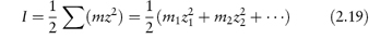
where the summation is continued over all the different species in solution. It can readily be shown from equation (2.19) that for a 1 : 1 electrolyte the ionic strength is equal to its molality; for a 1 : 2 electrolyte I = 3m; and for a 2 : 2 electrolyte I = 4m.
The Debye–Hückel expression as given by equation (2.18) is valid only in dilute solution (I < 0.02 mol kg–1). At higher concentrations a modified expression has been proposed:
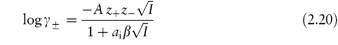
where ai is the mean distance of approach of the ions or the mean effective ionic diameter, and β is a constant whose value depends on the solvent and temperature. As an approximation, the product aiβ may be taken to be unity, thus simplifying the equation. Equation (2.20) is valid for I < 0.1 mol kg–1.
|
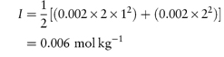
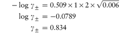
Calculate the mean ionic activity coefficient of: (a) 0.002 mol kg−1 aqueous solution of ephedrine sulfate; (b) an aqueous solution containing 0.002 mol kg−1 ephedrine sulfate and 0.01 mol kg−1 sodium chloride. Both solutions are at 25°C. Answer (a) Ephedrine sulfate is a 1:2 electrolyte and hence the ionic strength is given by equation (2.19) as
From the Debye–Hückel equation (equation 2.18),
(b) Ionic strength of 0.01 mol kg−1 NaCl = ½(0.01 × 12) + (0.01 × 12) = 0.01 mol kg−1
|

2.3.3 Solvent activity
Although the phrase ‘activity of a solution’ usually refers to the activity of the solute in the solution, as in the preceding section, we also can refer to the activity of the solvent. Experimentally, solvent activity a1 may be determined as the ratio of the vapour pressure p1 of the solvent in a solution to that of the pure solvent  , that is,

where γ1 is the solvent activity coefficient and x1 is the mole fraction of solvent.
The relationship between the activities of the components of the solution is expressed by the Gibbs–Duhem equation:

which provides a way of determining the activity of the solute from measurements of vapour pressure. An example of the role of water activity in inhibiting bacterial growth in wounds is given below.
Water activity and inhibition of bacterial growth
When thinking about the role of water activity in determining bacterial growth it is useful, but not strictly correct, to picture water activity as a measure of the amount of ‘available’ water in a system; this is not the total amount but the quantity that is free to act as a solvent. Some of the water may be unavailable because it is bound, either chemically or physically, to solutes present in the system; this water has different properties to free water and is biologically unavailable for microbial growth. Consequently, when the aqueous solution in the environment of a microorganism is concentrated by the addition of solutes such as sucrose, the consequences for microbial growth result mainly from a change in the amount of free water which is reflected in a change in the water activity aw. Every microorganism has a limiting aw below which it will not grow. The minimum aw levels for growth of human bacterial pathogens such as streptococci, Klebsiella, Escherichia coli, Corynebacterium, Clostridium perfringens and other clostridia, and Pseudomonas is 0.91.4 Staphylococcus aureus can proliferate at an aw as low as 0.86. Figure 2.2 shows the influence of aw, adjusted by the addition of sucrose, on the growth rate of this microorganism at 35°C and pH 7.0. The control medium, with a water activity value of aw = 0.993, supported the rapid growth of the test organism. Reduction of aw of the medium by addition of sucrose progressively increased generation times and lag periods and lowered the peak cell counts. Complete growth inhibition was achieved at an aw of 0.858 (195 g sucrose per 100 g water) with cell numbers declining slowly throughout the incubation period.
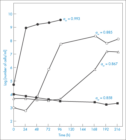
Figure 2.2 Staphylococcal growth at 35°C in medium alone (aw = 0.993) and in media with aw values lowered by additional sucrose.
Reproduced with permission from Chirife J et al. Scientific basic for use of granulated sugar in treatment of infected wounds. Lancet 1982;319:560–561.
These results explain why the old remedy of treating infected wounds with sugar, honey or molasses is successful. When the wound is filled with sugar, the sugar dissolves in the tissue water, creating an environment of low aw, which inhibits bacterial growth. However, the difference in water activity between the tissue and the concentrated sugar solution causes migration of water out of the tissue, hence diluting the sugar and raising aw. Further sugar must then be added to the wound to maintain growth inhibition. Sugar may be applied as a paste with a consistency appropriate to the wound characteristics; thick sugar paste is suitable for cavities with wide openings, whereas a thinner paste with the consistency of thin honey is more suitable for instillation into cavities with small openings. |

An in vitro study has been reported5 of the efficacy of thick sugar pastes, and also of those prepared using xylose as an alternative to sucrose, in inhibiting the growth of bacteria commonly present in infected wounds. Polyethylene glycol was added to the pastes as a lubricant and hydrogen peroxide was included in the formulation as a preservative. To simulate the dilution that the pastes invariably experience as a result of fluid being drawn into the wound, serum was added to the formulations in varying amounts. Figure 2.3 illustrates the effects of these sucrose pastes on the colony-forming ability of Proteus mirabilis and shows the reduction in efficiency of the pastes as a result of dilution and the consequent increase of their water activity from a value of 0.50 at 90% to 0.86 at 50% v/v paste in serum. It is clear that P. mirabilis was susceptible to the antibacterial activity of the pastes, even when they were diluted by 50%. It was reported that, although aw may not be maintained at less than 0.86 (the critical level for inhibition of growth of S. aureus) for more than 3 h after packing of the wound, nevertheless clinical experience had shown that twice-daily dressing was adequate to remove infected slough from dirty wounds within a few days.
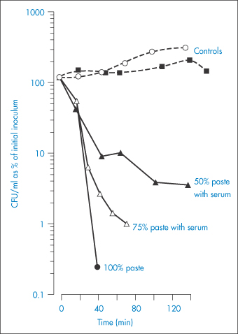
Figure 2.3 The effects of sucrose pastes diluted with serum on the colony-forming ability in Colony Forming Units (CFU) of Proteus mirabilis.
Reproduced with permission from Ambrose U et al. In vitro studies of water activity and bacterial growth inhibition of sucrose-polyethylene glycol 400-hydrogen peroxide and xylose-polyethylene glycol 400-hydrogen peroxide pastes used to treat infected wounds. Antimicrob Agents Chemother 1991;35:1799–1803.
Water activity and assessment of pharmaceutical products
As we have discussed above, there is a link between water activity and microbial growth. However, because water activity can be thought of as a measure of the free (i.e. unbound) water in the system, it also indicates the ability of water to act as a solvent and to migrate within the system; this has several other implications relating to, for example, chemical degradation, dissolution of solids and moisture-induced phase changes such as those which occur in amorphous systems. Consequently, the measurement of the total water content by, for example, Karl Fischer analysis does not provide information on the ‘availability’ of the water; determination of the water activity would enable better correlations to biological and chemical reaction rates within the formulation. Despite this, there is a currently a general reluctance to utilise water activity measurements in the assessment of pharmaceutical products. Recent guidance provided by the regulatory bodies’ International Conference on Harmonisation may provide an impetus to begin effectively using water activity in pharmaceutical quality programs.6
2.3.4 Chemical potential
Properties such as volume, enthalpy, free energy and entropy that depend on the quantity of substance are called extensive properties. In contrast, properties such as temperature, density and refractive index that are independent of the amount of material are referred to as intensive properties. The quantity denoting the rate of increase in the magnitude of an extensive property with increase in the number of moles of a substance added to the system at constant temperature and pressure is termed a partial molar quantity. Such quantities are distinguished by a bar above the symbol for the particular property. For example:
Note the use of the symbol ∂ to denote a partial change, which, in this case, occurs under conditions of constant temperature, pressure and number of moles of solvent (denoted by the subscripts outside the brackets).
In practical terms the partial molar volume,  , represents the change in the total volume of a large amount of solution when one additional mole of solute is added – it is the effective volume of 1 mole of solute in solution.
Of particular interest is the partial molar free energy,  , which is also referred to as the chemical potential, μ, and is defined for component 2 in a binary system by
Partial molar quantities are of importance in the consideration of open systems, that is, those involving transference of matter as well as energy. For an open system involving two components,
At constant temperature and pressure equation (2.25) reduces to

Thus,
The chemical potential therefore represents the contribution per mole of each component to the total free energy. It is the effective free energy per mole of each component in the mixture and is always less than the free energy of the pure substance.
It can be readily shown (see Derivation Box 2D) that the chemical potential of a component in a two-phase system (for example, oil and water) at equilibrium at a fixed temperature and pressure is identical in both phases, i.e.

where a and b are two immiscible phases.
Because of the need for equality of chemical potential at equilibrium, a substance in a system that is not at equilibrium will have a tendency to diffuse spontaneously from a phase in which it has a high chemical potential to another in which it has a low chemical potential. In this respect, the chemical potential resembles electrical potential and hence its name is an apt description of its nature.
Chemical potential of a component in solution
Where the component of the solution is a non-electrolyte, its chemical potential in dilute solution at a molality m can be calculated from

where

and M1 is the molecular weight of the solvent.
At higher concentrations, the solution generally exhibits significant deviations from ideality and the concentration must be replaced by activity

In the case of strong electrolytes, the chemical potential is the sum of the chemical potential of the ions. For the simple case of a 1 : 1 electrolyte, the chemical potential is given by

The derivations of these equations are given in Derivation Box 2E.
|
|

2.4 Osmotic properties of drug solutions
A non-volatile solute added to a solvent affects not only the magnitude of the vapour pressure above the solvent but also the freezing point and the boiling point to an extent that is proportional to the relative number of solute molecules present, rather than to the weight concentration of the solute. Properties that are dependent on the number of molecules in solution in this way are referred to as colligative properties, and the most important of such properties from a pharmaceutical viewpoint is the osmotic pressure.
2.4.1 Osmotic pressure
Whenever a solution is separated from a solvent by a membrane that is permeable only to solvent molecules (referred to as a semipermeable membrane), there is a passage of solvent across the membrane into the solution. This is the phenomenon of osmosis. If the solution is totally confined by a semipermeable membrane and immersed in the solvent, a pressure differential develops across the membrane, which is referred to as the osmotic pressure. Solvent passes through the membrane because of the inequality of the chemical potentials on either side of the membrane. Since the chemical potential of a solvent molecule in solution is less than that in pure solvent, solvent will spontaneously enter the solution until this inequality is removed. The equation that relates the osmotic pressure of the solution, Π, to the solution concentration is the van’t Hoff equation:

On application of the van’t Hoff equation to the drug molecules in solution, consideration must be made of any ionisation of the molecules, since osmotic pressure, being a colligative property, will be dependent on the total number of particles in solution (including the free counterions). To allow for what was at the time considered to be anomalous behaviour of electrolyte solutions, van’t Hoff introduced a correction factor, i. The value of this factor approaches a number equal to that of the number of ions, ν, into which each molecule dissociates as the solution is progressively diluted. The ratio i/ν is termed the practical osmotic coefficient,  .
.
For non-ideal solutions, the activity and osmotic pressure are related by the expression
where M1 is the molecular weight of the solvent and m is the molality of the solution. The relationship between the osmotic pressure and the osmotic coefficient is thus
where  is the partial molal volume of the solvent.
2.4.2 Osmolality and osmolarity
The experimentally derived osmotic pressure is frequently expressed as the osmolality ξm, which is the mass of solute that when dissolved in 1 kg of water will exert an osmotic pressure, Π′, equal to that exerted by a mole of an ideal un-ionised substance dissolved in 1 kg of water. The unit of osmolality is the osmole (abbreviated as osmol), which is the amount of substance that dissociates in solution to form one mole of osmotically active particles, thus 1 mole of glucose (not ionised) forms 1 osmole of solute, whereas 1 mole of NaCl forms 2 osmoles (1 mole of Na+ and 1 mole of Cl−). In practical terms, this means that a 1 molal solution of NaCl will have (approximately) twice the osmolality (osmotic pressure) as a 1 molal solution of glucose.
According to the definition ξm = Π/Π′, the value of Π′ may be obtained from equation (2.33) by noting that, for an ideal un-ionised substance ν =  = 1, and since m is also unity, equation (2.33) becomes
Thus

|
A 0.90% w/w solution of sodium chloride (mol wt = 58.5 Da) has an osmotic coefficient of 0.928. Calculate the osmolality of the solution. Answer Osmolality is given by equation (2.34) as
so
|


Pharmaceutical labelling regulations sometimes require a statement of the osmolarity; for example, the USP 27 requires that sodium chloride injection should be labelled in this way. Osmolarity is defined as the mass of solute which, when dissolved in 1 litre of solution, will exert an osmotic pressure equal to that exerted by a mole of an ideal un-ionised substance dissolved in 1 litre of solution. The relationship between osmolality and osmolarity has been discussed by Streng et al.7
Table 2.1 lists the osmolalities of commonly used intravenous (IV) fluids.
Table 2.1 Tonicities (osmolalities) of intravenous fluids
Solution | Tonicity (mosmol kg−1) |
Vamin 9 | 700 |
Vamin 9 Glucose | 1350 |
Vamin 14 | 1145 |
Vamin 14 Electrolyte-free | 810 |
Vamin 18 Electrolyte-free | 1130 |
Vaminolact | 510 |
Vitrimix KV | 1130 |
Intralipid 10% Novum | 300 |
Intralipid 20% | 350 |
Intralipid 30% | 310 |
Intrafusin 22 | 1400 |
Hyperamine 30 | 1450 |
Gelofusine | 279a |
Lipofundin MCT/LCT 10% | 345a |
Lipofundin MCT/LCT 20% | 380a |
Nutriflex 32 | 1140a |
Nutriflex 48 | 1400a |
Nutriflex 70 | 2100a |
Sodium Bicarbonate Intravenous Infusion BP | |
8.4% w/v | 2000a |
4.2% w/v | 1000a |
a Osmolarity (mosmol dm−3).
2.4.3 Clinical relevance of osmotic effects
Tonicity
Osmotic effects are particularly important from a physiological viewpoint since biological membranes, notably the red blood cell membrane, behave in a manner similar to that of semipermeable membranes. Consequently, when red blood cells are immersed in a solution of greater osmotic pressure than that of their contents, they shrink as water passes out of the cells in an attempt to reduce the chemical potential gradient across the cell membrane. Conversely, on placing the cells in an aqueous environment of lower osmotic pressure, the cells swell as water enters and eventually lysis may occur. It is an important consideration, therefore, to ensure that the effective osmotic pressure of a solution for injection is approximately the same as that of blood serum. This effective osmotic pressure, which is termed the tonicity, is not always identical to the osmolality because it is concerned only with those solutes in solution that can exert an effect on the passage of water through the biological membrane. Solutions that have the same tonicity as blood serum are said to be isotonic with blood. Solutions with a higher tonicity are hypertonic and those with a lower tonicity are termed hypotonic solutions. Similarly, in order to avoid discomfort on administration of solutions to the delicate membranes of the body, such as the eyes, these solutions are made isotonic with the relevant tissues.
The osmotic pressures of many of the products in Table 2.1 are in excess of that of plasma (291 mosmol dm−3). It is generally recommended that any fluid with an osmotic pressure above 550 mosmol dm−3 should not be infused rapidly as this would increase the incidence of venous damage. The rapid infusion of marginally hypertonic solutions (in the range 300–500 mosmol dm−3) would appear to be clinically practicable; the higher the osmotic pressure of the solution within this range, the slower should be its rate of infusion to avoid damage. Patients with centrally inserted lines are not normally affected by limits on tonicity as infusion is normally slow and dilution is rapid.
Certain oral medications commonly used in the intensive care of premature infants have very high osmolalities. The high tonicity of enteral feedings has been implicated as a cause of necrotising enterocolitis (NEC). A higher frequency of gastrointestinal illness including NEC has been reported8 among premature infants fed undiluted calcium lactate than among those fed no supplemental calcium or calcium lactate diluted with water or formula. White and Harkavy9 have discussed a similar case of the development of NEC following medication with calcium glubionate elixir. |

White and Harkavy9 have measured osmolalities of several medications by freezing-point depression and compared these with the osmolalities of analogous IV preparations (Table 2.2). Except in the case of digoxin, the osmolalities of the IV preparations were very much lower than those of the corresponding oral preparations despite the fact that the IV preparations contained at least as much drug per millilitre as did the oral forms. This striking difference may be attributed to the additives such as ethyl alcohol, sorbitol and propylene glycol, which make a large contribution to the osmolalities of the oral preparations. The vehicle for the IV digoxin consists of 40% propylene glycol and 10% ethyl alcohol with calculated osmolalities of 5260 and 2174 mosmol kg−1 respectively, thus explaining the unusually high osmolality of this IV preparation. These authors have recommended that extreme caution should be exercised in paediatric and neonatal therapy in the administration of these oral preparations and perhaps any medication in a syrup or elixir form when the infant is at risk from NEC.
Table 2.2 Measured and calculated osmolalities of drugs
Drug (route) | Concentration of drug | Mean measured osmolality (mosmol kg−1) | Calculated available milliosmoles in 1 kg of drug preparationa |
Theophylline elixir (oral) | 80 mg/15 cm3 | >3000 | 4980 |
Aminophylline (IV) | 25 mg cm−3 | 116 | 200 |
Calcium glubionate (oral) | 115 mg/5 cm3 | >3000 | 2270 |
Calcium gluceptate (IV) | 90 mg/5 cm3 | 507 | 950 |
Digoxin elixir | 25 mg dm−3 | >3000 | 4420 |
Digoxin (IV) | 100 mg dm−3 | >3000 | 9620 |
Dexametasone elixir (oral) | 0.5 mg/5 cm3 | >3000 | 3980 |
Dexametasone sodium phosphate (IV) | 4 mg cm−3 | 284 | 312 |
aThis would be the osmolality of the drug if the activity coefficient were equal to 1 in the full-strength preparation. The osmolalities of serial dilutions of the drug were plotted against the concentrations of the solution, and a least-squares regression line was drawn. The value for the osmolality of the full-strength solution was then estimated from the line. This is the ‘calculated available milliosmoles’.
Reproduced with permission from White KC, Harkavy KL (1982). Hypertonic formula resulting from added oral medications. Am J Dis Child; 136:931–933.
The osmolarity of preparations for oral administration to premature infants should be less than 400–500 mosmol dm−3 to limit stress imposed on the gastrointestinal system, which could lead to pneumatosis intestinalis.10 Many drugs administered to preterm infants, however, have osmolarities greatly exceeding this limit, for example, paracetamol (acetaminophen) solutions have osmolarities of 10 000–16 000 mosmol dm−3. |

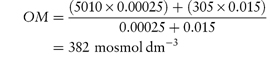
Where no suitable alternative drugs are available, it may be possible to reduce osmolarity by administering the drugs by mixing with an infant formula. In such cases the final osmolarity of the mixture (OM) is calculated from
where OD and OF are the osmolarities of drug and infant formula, respectively, and VD and VF are the volumes of drug solution and infant formula, respectively. Example 2.4 (taken from reference 10) illustrates the use of this equation.
|
A 0.25 mL solution of Fer-In-Sol drops has an approximate osmolarity of 5010 mosmol dm−3; calculate the final osmolarity of the preparation obtained when this dose is added to 15 mL of Premature Enfamil Formula (osmolarity 305 mosmol dm−3). Answer Substitution in equation (2.35) gives
Note that the volumes are converted to litres (dm−3) before substitution. |

In some cases the osmolality of the elixir is so high that even mixing with infant formula does not reduce the osmolality to a tolerable level. For example, when a clinically appropriate dose of dexamethasone elixir was mixed in volumes of formula appropriate for a single feeding for a 1500 g infant, the osmolalities of the mixes increased by at least 300% compared to formula alone (Table 2.3).
Table 2.3 Osmolalities of drug–infant formula mixtures
Drug (dose) | Volume of drug (cm3) + volume of formula (cm3) | Mean measured osmolality (mosmol kg−1) |
Infant formula | – | 292 |
Theophylline elixir, 1 mg kg−1 | 0.3 + 15 | 392 |
0.3 + 30 | 339 | |
Calcium glubionate syrup, 0.5 mmol kg−1 | 0.5 + 15 | 378 |
0.5 + 30 | 330 | |
Digoxin elixir, 5 μg kg−1 | 0.15 + 15 | 347 |
0.15 + 30 | 322 | |
Dexamethasone elixir, 0.25 mg kg−1 | 3.8 + 15 | 1149 |
3.8 + 30 | 791 |
Reproduced with permission from White KC, Harkavy KL (1982). Hypertonic formula resulting from added oral medications. Am J Dis Child; 136:931–933.
Volatile anaesthetics
The aqueous solubilities of several volatile anaesthetics can be related to the osmolarity of the solution.11 The inverse relationship between solubility (expressed as the liquid/gas partition coefficient) of those anaesthetics and the osmolarity is shown in Table 2.4.
Table 2.4 Liquid/gas partition coefficients of anaesthetics in four aqueous solutions at 37°C
Solution | Osmolarity (mosmol dm−3) | Partition coefficient | |||
Isoflurane | Enflurane | Halothane | Methoxyflurane | ||
Distilled H2O | 0 | 0.626 ± 0.05 | 0.754 ± 0.06 | 0.859 ± 0.02 | 4.33 ± 0.5 |
Normal saline | 308 | 0.590 ± 0.01 | 0.713 ± 0.01 | 0.825 ± 0.02 | 4.22 ± 0.30 |
Isotonic heparin (1000 U cm−3) | 308 | 0.593 ± 0.01 | 0.715 ± 0.01 | – | 4.08 ± 0.22 |
Mannitol (20%) | 1098 | 0.476 ± 0.023 | 0.575 ± 0.024 | 0.747 ± 0.03 | 3.38 ± 0.14 |
Reproduced with permission from Lerman J et al. Osmolarity determines the solubility of anesthetics in aqueous solutions at 37°C. Anesthesiology 1983;59:554–558.
These findings have practical applications for the clinician. Although changes in serum osmolarity within the physiological range (209–305 mosmol dm−3) have only a small effect on the liquid/gas partition coefficient, changes in the serum osmolarity and the concentration of serum constituents at the extremes of the physiological range may significantly decrease the liquid/gas partition coefficient. For example, the blood/gas partition coefficient of isoflurane decreases significantly after an infusion of mannitol. This decrease may be attributed to both a transient increase in the osmolarity of the blood and a more prolonged decrease in the concentration of serum constituents caused by the influx of water due to the osmotic gradient.
Rehydration solutions
An interesting application of the osmotic effect has been in the design of rehydration solutions. During the day the body moves many litres of fluid from the blood into the intestine and back again. The inflow of water into the intestine, which aids the breakdown of food, is an osmotic effect arising from the secretion of Cl− ions by the crypt cells of the intestinal lining (see section 8.2.2) into the intestine. Nutrients from the food are taken up by the villus cells in the lining of the small intestine. The villus cells also absorb Na+ ions, which they pump out into the extracellular spaces, from where they return to the circulation. As a consequence of this flow of Na+, water and other ions follow by osmotic flow and hence are also transferred to the blood. This normal functioning is disrupted by diarrhoea-causing microorganisms, which either increase the Cl−-secreting activity of the crypt cells or impair the absorption of Na+ by the villus cells, or both. Consequently, the fluid that is normally returned to the blood across the intestinal wall is lost in watery stool. If untreated, diarrhoea can eventually lead to a severe decline in the volume of the blood, the circulation may become dangerously slow, and death may result.
Oral rehydration therapy
Treatment of dehydration by oral rehydration therapy (ORT) is based on the discovery that the diarrhoea-causing organisms do not usually interfere with the carrier systems that bring sodium and glucose simultaneously into the villus cells from the intestinal cavity. This ‘co-transport’ system only operates when both sodium and glucose are present. The principle behind ORT is that if glucose is mixed into an electrolyte solution it activates the co-transport system, causing electrolyte and then water to pass through the intestinal wall and to enter the blood, so minimising the dehydration.
ORT requires administration to the patient of small volumes of fluid throughout the day (to prevent vomiting); it does not reduce the duration or severity of the diarrhoea, it simply replaces lost fluid and electrolytes. Let us examine, using the principles of the osmotic effect, two possible methods by which the process of fluid uptake from the intestine might be speeded up. It might seem reasonable to suggest that more glucose should be added to the formulation in an attempt to enhance the co-transport system. If this is done, however, the osmolarity of the glucose will become greater than that of normal blood, and water would now flow from the blood to the intestine and so exacerbate the problem. An alternative is to substitute starches for simple glucose in the ORT. When these polymer molecules are broken down in the intestinal lumen, they release many hundreds of glucose molecules, which are immediately taken up by the co-transport system and removed from the lumen. The effect is therefore as if a high concentration of glucose were administered, but because osmotic pressure is a colligative property (dependent on the number of molecules rather than the mass of substance), there is no associated problem of a high osmolarity when starches are used. The process is summarised in Fig. 2.4. A similar effect is achieved by the addition of proteins, since there is also a co-transport mechanism whereby amino acids (released on breakdown of the proteins in the intestine) and Na+ ions are simultaneously taken up by the villus cells.
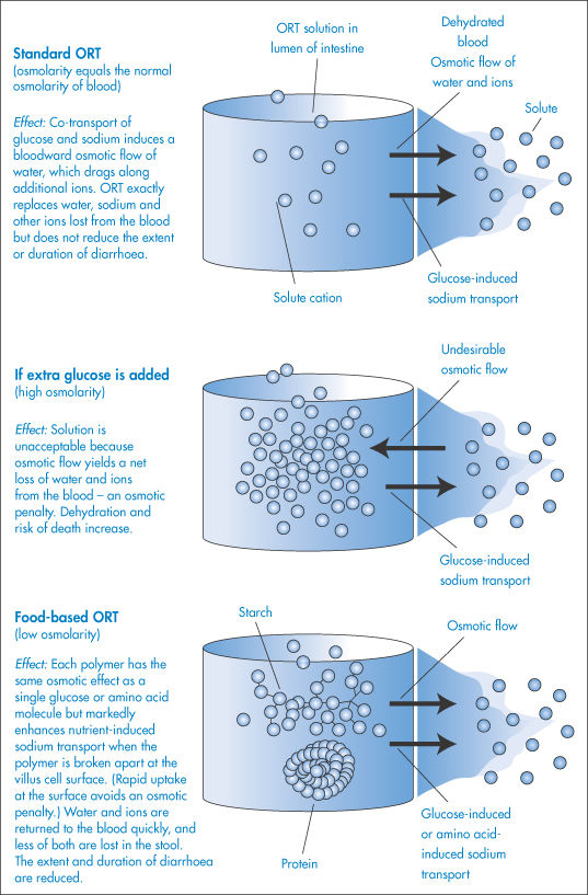
Figure 2.4 How osmosis affects the performance of solutions used in oral rehydration therapy (ORT).
This process of increasing water uptake from the intestine has an added appeal since the source of the starch and protein can be cereals, beans and rice, which are likely to be available in the parts of the world where problems arising from diarrhoea are most prevalent. Food-based ORT offers additional advantages: it can be made at home from low-cost ingredients and can be cooked, which kills the pathogens in the water.
2.4.4 Preparation of isotonic solutions
Since osmotic pressure is not a readily measurable quantity, it is usual to make use of the relationship between the colligative properties and to calculate the osmotic pressure from a more easily measured property such as the freezing-point depression. In so doing, however, it is important to realise that the red blood cell membrane is not a perfect semipermeable membrane and allows through small molecules such as urea and ammonium chloride. Therefore, although the quantity of each substance required for an isotonic solution may be calculated from freezing-point depression values, these solutions may cause cell lysis when administered.
It has been shown that a solution that is isotonic with blood has a freezing-point depression, ΔTf, of 0.52°C. One has therefore to adjust the freezing point of the drug solution to this value to give an isotonic solution. Freezing-point depressions for a series of compounds are given in reference texts1,12 and it is a simple matter to calculate the concentration required for isotonicity from these values. For example, a 1% NaCl solution has a freezing-point depression of 0.576°C. The percentage concentration of NaCl required to make isotonic saline solution is therefore (0.52/0.576) × 1.0 = 0.90% w/v.
With a solution of a drug, it is of course not possible to alter the drug concentration in this manner, and an adjusting substance must be added to achieve isotonicity. The quantity of adjusting substance can be calculated as shown in Box 2.3.
Box 2.3 Preparation of isotonic solutions |
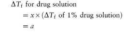
If the drug concentration is x g per 100 cm3 solution, then
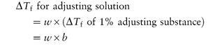
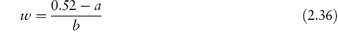
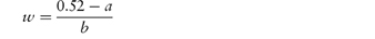
Similarly, if w is the weight in grams of adjusting substance to be added to 100 cm3 of drug solution to achieve isotonicity, then
For an isotonic solution, a + (w × b) = 0.52. Therefore,
|
|
Calculate the amount of sodium chloride that should be added to 50 cm3 of a 0.5% w/v solution of lidocaine hydrochloride to make a solution isotonic with blood serum. Answer From reference lists, the values of b for sodium chloride and lidocaine hydrochloride are 0.576°C and 0.130°C, respectively. From equation (2.36) we have
Hence,
Therefore, the weight of sodium chloride to be added to 50 cm3 of solution is 0.395 g. |


|
where w is the weight in grams of adjusting substance to be added to 100 mL of drug solution to achieve isotonicity, a is the number of grams of drug in 100 mL of solution multiplied by the freezing-point depression ΔTf of a 1% drug solution, and b is ΔTf of 1% adjusting substance. |

2.5 Ionisation of drugs in solution
Many drugs are either weak organic acids (for example, acetylsalicylic acid (aspirin)), or weak organic bases (for example, procaine), or their salts (for example, ephedrine hydrochloride). The degree to which these drugs are ionised in solution is highly dependent on the pH. The exceptions to this general statement are the non-electrolytes, such as the steroids, and the quaternary ammonium compounds, which are completely ionised at all pH values and in this respect behave as strong electrolytes.
2.5.1 Clinical relevance of drug ionisation
The extent of ionisation of a drug has an important effect on its absorption, distribution and elimination and there are many examples of the alteration of pH to change these properties. The pH of urine may be adjusted (for example, by administration of ammonium chloride or sodium bicarbonate) in cases of overdosing with amphetamines, barbiturates, narcotics and salicylates, to ensure that these drugs are completely ionised and hence readily excreted. Conversely, the pH of the urine may be altered to prevent ionisation of a drug in cases where reabsorption is required for therapeutic reasons. Sulfonamide crystalluria may also be avoided by making the urine alkaline. An understanding of the relationship between pH and drug ionisation is of use in the prediction of the causes of precipitation in admixtures, in the calculation of the solubility of drugs, and in the attainment of optimum bioavailability by maintaining a certain ratio of ionised to un-ionised drug. Table 2.5 shows the nominal pH values of some body fluids and sites, which are useful in the prediction of the percentage ionisation of drugs in vivo.
Table 2.5 Nominal pH values of some body fluids and sites
Site | Nominal pH |
Aqueous humour | 7.21 |
Blood, arterial | 7.4 |
Blood, venous | 7.39 |
Blood, maternal umbilical | 7.25 |
Cerebrospinal fluid | 7.35 |
Duodenum | 5.5 |
Faecesa | 7.15 |
Ileum, distal | 8.0 |
Intestine, microsurface | 5.3 |
Lacrimal fluid (tears) | 7.4 |
Milk, breast | 7.0 |
Muscle, skeletalb | 6.0 |
Nasal secretions | 6.0 |
Prostatic fluid | 6.45 |
Saliva | 6.40 |
Semen | 7.2 |
Stomach | 1.5 |
Sweat | 5.4 |
Urine, female | 5.8 |
Urine, male | 5.7 |
Vaginal secretions, premenopause | 4.5 |
Vaginal secretions, postmenopause | 7.0 |
Reproduced from Newton DW, Kluza RB. Drug Intell Clin Pharm 1978;12:547.
a Value for normal soft, formed stools; hard stools tend to be more alkaline, whereas watery, unformed stools are acidic.
b Studies conducted intracellularly in the rat.
2.5.2 Dissociation of weakly acidic and basic drugs and their salts
According to the Lowry–Brønsted theory of acids and bases, an acid is a substance that will donate a proton and a base is a substance that will accept a proton. Thus the dissociation of acetylsalicylic acid, a weak acid, could be represented as in Scheme 2.1. In this equilibrium, acetylsalicylic acid acts as an acid because it donates a proton, and the acetylsalicylate ion acts as a base because it accepts a proton to yield an acid. An acid and base represented by such an equilibrium is said to be a conjugate acid–base pair.
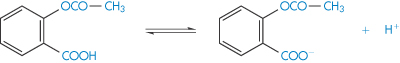
Scheme 2.1
Scheme 2.1 is not a realistic expression, however, since protons are too reactive to exist independently and are rapidly taken up by the solvent. The proton-accepting entity, by the Lowry–Brønsted definition, is a base, and the product formed when the proton has been accepted by the solvent is an acid. Thus a second acid–base equilibrium occurs when the solvent accepts the proton, and this may be represented by

The overall equation on summing these equations is shown in Scheme 2.2, or, in general,

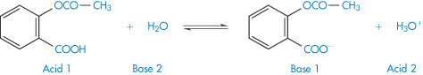
Scheme 2.2
By a similar reasoning, the dissociation of benzocaine, a weak base, may be represented by the equilibrium


or, in general,

Comparison of the two general equations shows that H2O can act as either an acid or a base. Such solvents are called amphiprotic solvents.
Salts of weak acids or bases are essentially completely ionised in solution. For example, ephedrine hydrochloride (salt of the weak base ephedrine, and the strong acid HCl) exists in aqueous solution in the form of the conjugate acid of the weak base, C6H5CH(OH)CH(CH3)N+H2CH3, together with its Cl− counterions. In a similar manner, when sodium salicylate (salt of the weak acid salicylic acid, and the strong base NaOH) is dissolved in water, it ionises almost entirely into the conjugate base of salicylic acid, HOC6H5COO−, and Na+ ions.
The conjugate acids and bases formed in this way are, of course, subject to acid–base equilibria described by the general equations above.
2.5.3 The effect of pH on the ionisation of weakly acidic or basic drugs and their salts
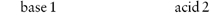
If the ionisation of a weak acid is represented as described above, we may express an equilibrium constant as follows:
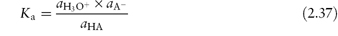
Assuming the activity coefficients approach unity in dilute solution, the activities may be replaced by concentrations:
Ka is variously referred to as the ionisation constant, dissociation constant or acidity constant for the weak acid. The negative logarithm of Ka is referred to as pKa, just as the negative logarithm of the hydrogen ion concentration is called the pH. Thus

Similarly, the dissociation constant or basicity constant for a weak base is
and

The pKa and pKb values provide a convenient means of comparing the strengths of weak acids and bases. The lower the pKa, the stronger the acid; the lower the pKb, the stronger is the base. The pKa values of a series of drugs are given in Table 2.6. pKa and pKb values of conjugate acid–base pairs are linked by the expression

Table 2.6 pKa values of some medicinal compoundsa
Compound | pKa | |
Acid | Base | |
Acebutolol |
| 9.4 |
Acetazolamide |
| 7.2, 9.0 |
Acetylsalicylic acid | 3.5 |
|
Aciclovir |
| 2.3, 9.3 |
Adrenaline | 9.9 | 8.5 |
Adriamycin |
| 8.2 |
Allopurinol | 10.2 |
|
Alphaprodine |
| 8.7 |
Alprazolam |
| 2.4 |
Alprenolol |
| 9.6 |
Amikacin |
| 8.1 |
p-Aminobenzoic acid | 4.9 | 2.4 |
Aminophylline |
| 5.0 |
p-Aminosalicylic acid | 3.2 |
|
Amitriptyline |
| 9.4 |
Compound | pKa | |
Acid | Base | |
Amiodorone |
| 6.6 (5.6)b |
Amoxicillin | 2.4 | 7.4, 9.6 |
Amoxapine |
| 7.6 |
Ampicillin | 2.7 | 7.2 |
Apomorphine | 8.9 | 7.0 |
Atenolol |
| 9.6 |
Ascorbic acid | 4.2, 11.6 |
|
Astemizole |
| 8.4 |
Atropine |
| 9.9 |
Azapropazone |
| 6.6 |
Azathioprine | 8.2 |
|
Azelastine |
| 9.5 |
Benazepril | 3.1 | 5.3 |
Benzylpenicillin | 2.8 |
|
Benzocaine |
| 2.8 |
Compound | pKa | |
Acid | Base | |
Bupivacaine |
| 8.1 |
Bupropion |
| 7.9 |
Captopril | 3.5 |
|
Carteolol |
| 9.7 |
Cefadroxil | 7.6 | 2.7 |
Cefalexin | 7.1 | 2.3 |
Cefaclor | 7.2 | 2.7 |
Celiprolol |
| 9.7 |
Cetirizine | 2.9 | 2.2, 8.0 |
Chlorambucil | 4.5 (4.9)b | 2.5 |
Chloramphenicol |
| 5.5 |
Chlorcyclizine |
| 8.2 |
Chlordiazepoxide |
| 4.8 |
Chloroquine |
| 8.1, 9.9 |
Chlorothiazide | 6.5 | 9.5 |
Chlorphenamine |
| 9.0 |
Chlorpromazine |
| 9.3 |
Chlorpropamide |
| 4.9 |
Chlorprothixene |
| 8.8 |
Cilazapril |
| 6.4 |
Cimetidine |
| 6.8 |
Cinchocaine |
| 8.3 |
Clarithromycin |
| 8.3 |
Clindamycin |
| 7.5 |
Cocaine |
| 8.5 |
Codeine |
| 8.2 |
Cyclopentolate |
| 7.9 |
Daunomycin |
| 8.2 |
Desipramine |
| 10.2 |
Dextromethorphan |
| 8.3 |
Diamorphine |
| 7.6 |
Diazepam |
| 3.4 |
Compound | pKa | |
Acid | Base | |
Dibucaine |
| 8.3 |
Diclofenac | 4.0 |
|
Diethylpropion |
| 8.7 |
Diltiazem |
| 8.0 |
Diphenhydramine |
| 9.1 |
Dithranol |
| 9.4 |
Doxepin |
| 8.0 |
Doxorubicin |
| 8.2,10.2 |
Doxycycline | 7.7 | 3.4, 9.3 |
Enalapril |
| 5.5 |
Enoxacin | 6.3 | 8.6 |
Epirubicin |
| 8.1 |
Ergometrine |
| 6.8 |
Ergotamine |
| 6.4 |
Erythromycin |
| 8.8 |
Famotidine |
| 6.8 |
Fenoprofen | 4.5 |
|
Flucloxacillin | 2.7 |
|
Flufenamic acid | 3.9 |
|
Flumequine | 6.5 |
|
Fluopromazine |
| 9.2 |
Fluorouracil | 8.0, 13.0 |
|
Fluphenazine |
| 3.9, 8.1 |
Flurazepam | 8.2 | 1.9 |
Flurbiprofen | 4.3 |
|
Furosemide | 3.9 |
|
Glibenclamide | 5.3 |
|
Guanethidine |
| 11.9 |
Guanoxan |
| 12.3 |
Halofantrine |
| 9.7 |
Haloperidol |
| 8.3 |
Hexobarbital | 8.3 |
|
Compound | pKa | |
Acid | Base | |
Hydralazine |
| 0.5, 7.1 |
Ibuprofen | 4.4 |
|
Imipramine |
| 9.5 |
Indometacin | 4.5 |
|
Ketoprofen | 4.0 |
|
Labetalol | 7.4 | 9.4 |
Levamisole |
| 8.0 |
Levodopa | 2.3, 9.7, 13.4 |
|
Lidocaine |
| 7.94 (26°C), 7.55 |
Lincomycin |
| 7.5 |
Loxoprofen | 4.2 |
|
Maprotiline |
| 10.2 |
Meclofenamic acid | 4.0 |
|
Metoprolol |
| 9.7 |
Methadone |
| 8.3 |
Methotrexate | 3.8, 4.8 | 5.6 |
Metronidazole |
| 2.5 |
Minocycline | 7.8 | 2.8, 5.0, 9.5 |
Minoxidil |
| 4.6 |
Morphine | 8.0 (phenol) | 9.6 (amine) |
Stay updated, free articles. Join our Telegram channel

Full access? Get Clinical Tree


