Figure 4.1 Diagrammatic representation of the three processes involved in the dissolution of a crystalline solute: the expression for the work involved is w22 + w11 − 2w12 (solute–solvent interaction in the last stage is −2w12 as bonds are made with one solute and two solvent molecules).
1. A solute (drug) molecule is ‘removed’ from its crystal.
2. A cavity for the molecule is created in the solvent.
3. The solute molecule is inserted into this cavity.
The first stage of the process involves the breaking of bonds within the crystal lattice, for example, overcoming the attractive electrostatic forces in a drug crystal consisting of cations and anions. The work required to achieve this may be written as w22; the subscript 2 is used for the solute and hence w22 implies solute–solute interaction. Work is also required in the creation of a cavity in the solvent to accommodate the displaced solute molecule; this may be written as w11 since now the process involves a solvent–solvent interaction (solvent is denoted by subscript 1). Placing the solute molecule in the solvent cavity requires a number of solute–solvent contacts; the larger the solute molecule, the more contacts are created. If the surface area of the solute molecule is A, the solute–solvent interface increases by σ12.A, where σ12 is the interfacial tension between the solvent and the solute. σ is a parameter not readily obtained for solid interfaces on the molecular scale, but reasonable estimates can be made from knowledge of the interfacial tensions of molecules at normal interfaces.1–5
The number of solvent molecules that can pack around the solute molecule is considered in calculations of the thermodynamic properties of the solution. The molecular surface area of the solute is therefore the key parameter and good correlations can be obtained between aqueous solubility and this parameter.4,5 Chain branching of hydrophobic groups also influences aqueous solubility, as shown by the solubilities of a series of straight and branched-chain alcohols in Table 4.1.
Table 4.1 Experimental aqueous solubilities, boiling points, surface areas and predicted aqueous solubilities
Compound | Solubility (mol kg−1) | Surface area (nm2) | Boiling point (°C) | Predicted solubilities (mol kg −1) |
1-Butanol | 1.006 | 2.721 | 117.7 | 0.821 |
1-Pentanol | 2.5 × 10⁻¹ | 3.039 | 137.8 | 2.09 × 10⁻¹ |
1-Hexanol | 6.1 × 10⁻² | 3.357 | 157 | 5.32 × 10⁻² |
1-Heptanol | 1.55 × 10⁻² | 3.675 | 176.3 | 1.36 × 10⁻² |
Cyclohexanol | 3.83 × 10⁻¹ | 2.905 | 161 | 4.3 × 10⁻¹ |
1-Nonanol | 1 × 10⁻³ | 4.312 | 213.1 | 0.88 × 10⁻³ |
Reproduced from Amidon GL et al. Solubility of nonelectrolytes in polar solvents. II. Solubility of aliphatic alcohols in water. J Pharm Sci 1974;63:1858–1866. Copyright Wiley-VCH Verlag GmbH & Co. KGaA. Reproduced with permission.
Of course, most drugs are not simple non-polar hydrocarbons and we have to consider polar molecules and weak organic electrolytes. The term w12 in Fig. 4.1, a measure of solute–solvent interactions, has to be further divided to take into account the interactions involving the non-polar part and the polar portion of the solute. The molecular surface area of each portion can be considered separately: the greater the area of the hydrophilic portion relative to the hydrophobic portion, the greater is the aqueous solubility. For a hydrophobic molecule of area A, the free-energy change in placing the solute in the solvent cavity is −σ12A. Indeed, it can be shown that the reversible work of solution is (w11 + w22 − 2w12)A.
Implicit in this derivation is the assumption that the solution formed is dilute, so that solute–solute interactions are unimportant. The success of the molecular area approach is evidenced by the fact that equations can be written to relate solubility to surface area. For example, equation (4.1) has been shown to hold for a range of 55 compounds (some of which are listed in Table 4.1):

where S is the molal (not molar) solubility, and A is the total surface area in nm2.
The compounds in Table 4.1 are liquids, so the process of dissolution is simpler than that outlined in Fig. 4.1.
Melting point and boiling point
Interactions between non-polar groups and water were discussed above, where the importance of both size and shape was indicated. What other predictors of solubility might there be? The boiling point of liquids and the melting point of solids are useful in that both reflect the strengths of interactions between the molecules in the pure liquid or the solid state. Boiling point correlates with total surface area, and in a large enough range of compounds we can detect the trend of decreasing aqueous solubility with increasing boiling point (see data in Table 4.2).
Table 4.2 Solubilities of pentanol isomers in water
Compound | Solubility (molality, m) | Surface area (nm2) | Boiling point (°C) | Structure |
1-Pentanol | 2.6 × 10⁻¹ | 3.039 | 137.8 |
|
3-Methyl-1-butanol | 3.11 × 10⁻¹ | 2.914 | 131.2 |
|
2-Methyl-1-butanol | 3.47 × 10⁻¹ | 2.894 | 128.7 |
|
2-Pentanol | 5.3 × 10⁻¹ | 2.959 | 119.0 |
|
3-Pentanol | 6.15 × 10⁻¹ | 2.935 | 115.3 |
|
3-Methyl-2-butanol | 6.67 × 10⁻¹ | 2.843 | 111.5 |
|
2-Methyl-2-butanol | 1.403 | 2.825 | 102.0 |
|


Reproduced from Amidon GL et al. Solubility of nonelectrolytes in polar solvents. II. Solubility of aliphatic alcohols in water. J Pharm Sci 1974;63:1858–1866. Copyright Wiley-VCH Verlag GmbH & Co. KGaA. Reproduced with permission.
As boiling points of liquids and melting points of solids are indicators of molecular cohesion, these can be useful indicators of trends in a series of similar compounds. There are other empirical correlations that are useful. Melting points, even of compounds that form non-ideal solutions, can be used as a guide to the order of solubility in a closely related series of compounds, as can be seen in the properties of sulfonamide derivatives listed in Table 4.3. Such correlations depend on the relatively greater importance of w22 in the solution process in these compounds.
Table 4.3 Correlation between melting points of sulfonamide derivatives and aqueous solubility
Compound | Melting point (°C) | Solubility |
Sulfadiazine | 253 | 1 g in 13 dm3 (0.077 g dm−3) |
Sulfamerazine | 236 | 1 g in 5 dm3 (0.20 g dm−3) |
Sulfapyridine | 192 | 1 g in 3.5 dm3 (0.29 g dm−3) |
Sulfathiazole | 174 | 1 g in 1.7 dm3 (0.59 g dm−3) |
The relationship between the molar solubility of a drug in water, Sw, at a temperature T (in kelvins), and the melting point Tm, for a non-ideal solution may be written as
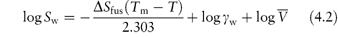
where  is the entropy of fusion (melting), γ is the activity coefficient and
  is the molar volume of the solvent. Equation (4.2) shows an increase of solubility as the melting point decreases.
Substituents
The influence of substituents on the solubility of molecules in water can be due to their effect on the properties of the solid or liquid (for example, on its molecular cohesion) or to the effect of the substituent on its interaction with water molecules. It is not easy to predict what effect a particular substituent will have on crystal properties, but as a guide to the solvent interactions, substituents can be classified as either hydrophobic or hydrophilic, depending on their polarity (Table 4.4). The position of the substituent on the molecule can influence its effect, however. This can be seen in the aqueous solubilities of o-, m– and p-dihydroxybenzenes; as expected, all are much greater than that of benzene, but they are not the same, being 4, 9 and 0.6 mol dm−3, respectively. The relatively low solubility of the para compound is due to its greater stability. The melting points of the derivatives indicate that is so, as they are 105°C, 111°C and 170°C, respectively. In the case of the ortho derivative, the possibility of intramolecular hydrogen bonding in aqueous solution, decreasing the ability of the OH group to interact with water, may explain why its solubility is lower than that of its meta analogue.
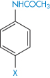
One can best illustrate the use of the information in Table 4.4 by considering the solubility of a series of substituted acetanilides, data for which are provided in Table 4.5. The strong hydrophilic characteristics of polar groups capable of hydrogen bonding with water molecules are evident. The presence of hydroxyl groups can therefore markedly change the solubility characteristics of a compound; phenol, for example, is 100 times more soluble in water than is benzene. In the case of phenol, where there is considerable hydrogen-bonding capability, the solute–solvent interaction (w12) outweighs other factors (such as w22 or w11) in the solution process. But, as we have discovered, the position of any substituent on the parent molecule will affect its contribution to solubility.
Table 4.4 Substituent group classification
Substituent | Classification |
‒CH3 | Hydrophobic |
‒CH2‒ | Hydrophobic |
‒Cl, ‒Br, ‒F | Hydrophobic |
‒N(CH3)2 | Hydrophobic |
‒SCH3 | Hydrophobic |
‒OCH2CH3 | Hydrophobic |
‒OCH3 | Slightly hydrophilic |
‒NO2 | Slightly hydrophilic |
‒CHO | Hydrophilic |
‒COOH | Slightly hydrophilic |
‒COO− | Very hydrophilic |
‒NH2 | Hydrophilic |
‒NH | Very hydrophilic |
‒OH | Very hydrophilic |

Table 4.5 The effect of substituents on solubility of acetanilide derivatives in water
Derivative | X | Solubility (mg dm−3) |
| H | 6.38 |
Methyl | 1.05 | |
Ethoxyl | 0.93 | |
Hydroxyl | 13.9 | |
Nitro | 15.98 | |
Aceto | 9.87 |
Steroid solubility
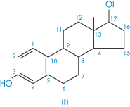
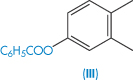
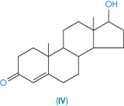
The steroids as a group tend to be poorly soluble in water. Their complex structure makes prediction of solubility somewhat difficult, but one can generally rationalise, post hoc, the solubility values of related steroids. Table 4.6 gives solubility data for 14 steroids. As examples, the substitution of an ethinyl group has conferred increased solubility on the estradiol molecule, as would be expected. Estradiol benzoate with its 3-OH substituent is much less soluble than the parent estradiol because of the loss of the hydroxyl and its substitution with a hydrophobic group. The same relationships are seen in testosterone and testosterone propionate. As both estradiol benzoate and testosterone propionate are oil soluble, they are used as solutions in castor oil and sesame oil for intramuscular and subcutaneous injection (see Chapter 9).
Table 4.6 Steroid structure and solubility in water
Structure | Compound | Solubility (μg cm−3) |
| Estradiol (I) | 5 |
| Ethinylestradiol (II) | 10 |
| Estradiol benzoate (III) | 0.4 |
| Testosterone (IV) | 24 0.4 |
| Methyltestosterone (V) | 32 |
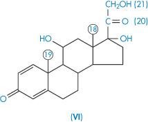
| Prednisolone (VI) | 215 |
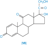
| Prednisone (VII) Prednisone acetate | 115 23 |
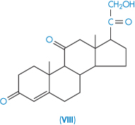
| Cortisone (VIII) | 230 |
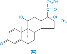
| Dexamethasone (IX) | 84 |
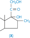
| Betamethasone (X) | 58 |
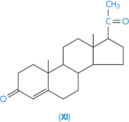
| Progesterone (XI) | 9 |
| Hydrocortisone (XII) | 285 |


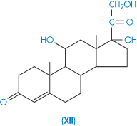
Reproduced from Kabasakalian P et al. Solubility of some steroids in water. J Pharm Sci 1966;55:642. Copyright Wiley-VCH Verlag GmbH & Co. KGaA. Reproduced with permission.
Methyltestosterone might be expected to be less soluble in water than is testosterone, but in fact it is not; this demonstrates again the importance of crystal properties in determining solubility. The methyl compound is more soluble because of the smaller heat of fusion of this derivative, hence the solid state more readily ‘disintegrates’ in the solvent.
Dexamethasone and betamethasone are isomeric fluorinated derivatives of methylprednisolone, but their solubilities are not identical, which might be a crystal property or a solution property. A simpler example of differences in isomeric solubility is that of the o-, m– and p-dihydroxybenzenes referred to above. A steric argument may be applied to the case of dexamethasone, water molecules being less able to move close to the 17-OH group than in the case of betamethasone.
4.2.2 Hydration and solvation
The way in which solute molecules interact with the water molecules of the solvent is crucial to determining their affinity for the solvent. Ionic groups and electrolytes interact avidly with the polar water molecules, but non-electrolytes also do not leave the structure of water unchanged, nor even do non-polar groups and molecules such as the hydrocarbons.
Hydration of non-electrolytes
Solvation is the general term used to describe the process of binding of solvent to solute molecules. If the solvent is water, the process is hydration. In a solution of sucrose (XIII), six water molecules are bound to each sucrose molecule with such avidity that the water and sucrose move as a unit in solution, and the extent of hydration can therefore be measured by hydrodynamic techniques.
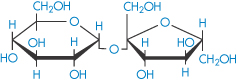
Structure XIII Sucrose
Chemically very similar molecules such as mannitol (XIV), sorbitol (XV) and inositol have very different affinities for water. The solubility of sorbitol in water is about 3.5 times that of mannitol.
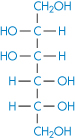
Structure XIV Mannitol
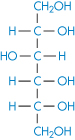
Structure XV Sorbitol
Most favourable hydration occurs when there is an equatorial –OH group on pyranose sugars.6 This is thought to be due to the compatibility of the equatorial –OH with the organised structure of water in bulk. Axial hydroxyl groups cannot bond on to the water ‘lattice’ without causing it to distort considerably. This may be one explanation of the difference, although differences in the lattice energies of the crystals may also contribute.
Hydration of ionic species: water structure breakers and structure makers
The study of ionic solvation is complicated but is relevant in pharmaceutics because of the effect ions have on the solubility of other species. The forces between cations and water molecules are so strong that the cations may retain a layer of water molecules in their crystals. The effect of ions on water structure is complex and variable. All ions in water possess a layer of tightly bound water – the water molecules being directionally oriented. Four water molecules are in the bound layer of most monovalent, monatomic ions. The firmly held layer can be regarded as being in a ‘frozen’ condition around a positive ion. The water molecules could be oriented with all the hydrogen atoms of the water molecules pointing outwards (Fig. 4.2). Because of this and because their orientation depends on the ion size, they cannot all participate in the normal tetrahedral arrangements of bulk water (see section 5.3.1 in Chapter 5). For this to be feasible, two of the water molecules must be oriented with the hydrogens of the water molecules pointing in towards the ion. Inevitably, then, with cations and many small anions there tends to be a layer of water around the bound layer which is less ordered than bulk water (Fig. 4.2). Such ions, which include all the alkali and halide ions except Li+ and F−, are called structure breakers. The size of the ion is important, as the surface area of the ion determines the constraints on the polarised water molecules. Many polyvalent ions, for example Al3+, increase the structured nature of water beyond the immediate hydration layer, and are therefore structure makers.
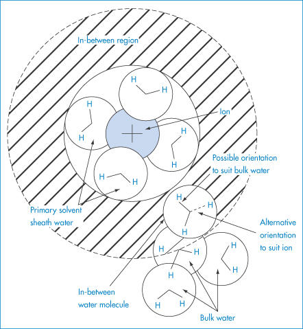
Figure 4.2 Schematic diagram to indicate that, in the (hatched) region between the primary solvated ion and bulk water, the orientation of the ‘in-between’ water molecules must be a compromise between that which suits the ion (oxygen-facing ion) and that which suits the bulk water (hydrogen-facing ion).
Reproduced with permission from Bockris JO’M, Reddy AKN. Modern Electrochemistry, vol. 1. London: MacDonald, 1970.
Hydration numbers
Hydration numbers (the number of water molecules in the primary hydration layer) can be determined by various physical techniques (for example, compressibility) and the values obtained tend to differ depending on the method used. The overall total action of the ion on water may be replaced conceptually by a strong binding between the ion and some effective number (solvation number) of solvent molecules; this effective number may well be almost zero in the case of large ions such as iodide, caesium and tetraalkylammonium ions. The solvation numbers decrease with increase of ionic radius because the ionic force field diminishes with increasing radius, and consequently water molecules are less inclined to be abstracted from their position in bulk water.
Hydrophobic hydration
Water is associated in a dynamic manner with non-polar groups, but only in rare cases (where crystalline clathrates can be formed) is this water able to be isolated along with the hydrophobic groups. The phrase ‘hydrophobic hydration’ is used to describe this layer of water. The motion of water molecules is slowed down in the vicinity of non-polar groups. Hydrophobic groups induce structure formation in water, hence the negative entropy (−ΔS) of their dissolution in water and the positive entropy (+ΔS) gained on their removal. In the discussion of hydrophobic bonding (see section 5.3.1 in Chapter 5) and non-polar interactions, this special relationship between water and hydrocarbon chains is elaborated.
The solubility of inorganic materials in water
While a minority of therapeutic agents are inorganic electrolytes, it is nevertheless pertinent to consider the manner of their interaction with water. Electrolytes are, of necessity, components of replacement fluids, injections and eye drops and many other formulations. An increasing number of metal-containing compounds are used in diagnosis and therapy, some of which have interesting solution behaviour.
First consider the simpler salts. What determines the solubility of a salt such as sodium chloride and its solubility in relation to, say, silver chloride? The solubility of NaCl is in excess of 5 mol dm−3 while the solubility of AgCl is 500 000 times less. The heats of solution (ΔHsolution) are 62.8 kJ mol−1 for silver chloride and 4.2 kJ mol−1 for sodium chloride, suggesting a substantial difference either in the crystal properties or in the interaction of the ions with water. In fact the very great strength of the silver chloride crystal is due to the high polarisability of the silver ion. The heat of solution of an ionic solute can be written as

Conceptually, the solid salt (sodium chloride, for instance) is converted to the gaseous (g) state, Na+(g) + Cl−(g), and each unit is then hydrated to form the species Na+(aq) and Cl−(aq). If the heat of hydration is sufficient to provide the energy needed to overcome the lattice forces, the salt will be freely soluble at a given temperature and the ions will readily dislodge from the crystal lattice. If the partial molal enthalpy of solution of the substance is positive, the solubility will increase with increasing temperature; if it is negative the solubility will decrease, in agreement with Le Chatelier’s principle.
4.2.3 The effect of simple additives on solubility
Solubility products
For poorly soluble materials such as silver chloride and barium sulfate the concept of the solubility product can be used. The following equilibrium exists in solution between crystalline silver chloride AgClc and ions in solution:

An equilibrium constant K can be defined as
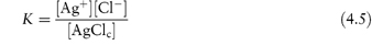
Strictly, K should be written in terms of thermodynamic activities and not concentrations, but activities can be replaced by concentrations (denoted by square brackets) because of the low solubilities involved (see section 2.3.1 in Chapter 2). At saturation the concentration of the crystalline silver chloride [AgClc] is essentially constant and the solubility product, Ksp, may therefore be written

The sparingly soluble compound silver chloride is an example of a 1 : 1 salt, i.e. each molecule ionises to give one ion of Ag+ and one of Cl−. When a compound has more than one ion of each type, for example, the poorly soluble salt calcium hydroxide Ca(OH)2, then the solubility product is defined as the product of each ion raised to the appropriate power. Calcium hydroxide ionises to give one ion of Ca2+ and two OH− ions and the solubility product becomes

Some values of solubility products are quoted in Table 4.7.
Table 4.7 Solubility products of some inorganic salts
Compound | Ksp (mol2 dm−6) |
AgCl | 1.25 × 10⁻¹⁰ |
Al(OH)3 | 7.7 × 10⁻¹³ |
BaSO4 | 1.0 × 10⁻¹⁰ |
Common ion effect
The solubility product is useful for evaluating the influence of other species on the solubility of salts of low aqueous solubility. One of the most important influences on the solubility of poorly soluble salts occurs on addition of another compound that has an identical ion to one of those of the salt. For example, if sodium chloride is added to a saturated solution of silver chloride, the concentration of Cl− ions in solution will be increased, as therefore will the product [Ag+][Cl−]. Consequently, to maintain Ksp constant the concentration of Ag+ in solution will decrease, i.e. solid AgCl will be precipitated. This effect, whereby the solubility of a sparingly soluble salt is decreased by the addition of another compound having an ion in common, is referred to as the common ion effect. Several examples of the influence of the common ion effect on drug solubilities in vivo are discussed in section 4.7.2.
Salting in and salting out
In general, additives may either increase or decrease the solubility of a solute in a given solvent. The effect that they have will depend on several factors:
- the effect the additive has on the structure of water
- the interaction of the additive with the solute
- the interaction of the additive with the solvent.
The effect of a solute additive on the solubility of another solute may be quantified by the Setschenow equation:
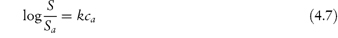
where Sa is the solubility in the presence of an additive, S is the solubility in its absence, ca is the concentration of additive and k is the salting coefficient. The sign of k is positive when the activity coefficient is increased; it is negative if the activity coefficient is decreased by the additive. The Setschenow equation frequently holds up to additive concentrations of 1 mol dm−3, a measure of the sensitivity of the activity coefficient of the solute towards the salt.
Salts that increase solubility are said to salt in the solute and those that decrease solubility salt out the solute. Salting out may result from the removal of water molecules that can act as solvent because of competing hydration of the added ion. The opposite effect, salting in, can occur when salts with large anions or cations that are themselves very soluble in water are added to the solutions of non-electrolytes. Sodium benzoate and sodium p-toluenesulfonate are good examples of such agents and are referred to as hydrotropic salts; the increase in the solubility of other solutes is known as hydrotropy. Values of k (in (mol dm−3)−1) for three salts added to benzoic acid in aqueous solution are 0.17 for NaCl; 0.14 for KCl; and −0.22 for sodium benzoate. That is, NaCl and KCl decrease the solubility of benzoic acid, and sodium benzoate increases it.
4.2.4 The effect of pH on the solubility of ionisable drugs
pH is one of the primary influences on the solubility of most drugs that contain ionisable groups. As the great majority of drugs are organic electrolytes, there are four parameters that determine their solubility:
1. their degree of ionisation
2. their molecular size
3. interactions of substituent groups with solvent
4. their crystal properties.
In this section consideration is given to the solubility of weak electrolytes and the influence of pH on aqueous solubility, important in both formulation and dissolution of drugs in vivo, and ultimately and importantly their biological activity.
Acidic drugs
Acidic drugs, such as the non-steroidal anti-inflammatory agents, are less soluble in acidic solutions than in alkaline solutions because the predominant undissociated species cannot interact with water molecules to the same extent as the ionised form, which is readily hydrated. Equation (4.8), which is a form of the Henderson–Hasselbalch equation relating drug solubility to the pH of the solution and to the pKa of the drug, is derived in Derivation Box 4A.
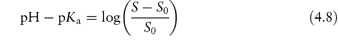
where S is the total saturation solubility of the drug and S0 is the solubility of the undissociated species. Examples of the use of equation (4.8) to calculate the effect of pH on the solubility of acidic drugs are given below.
|
What is the pH below which sulfadiazine (pKa = 6.48) will begin to precipitate in an infusion fluid, when the initial molar concentration of sulfadiazine sodium is 4 × 10⁻² mol dm−3 and the solubility of sulfadiazine is 3.07 × 10⁻⁴ mol dm−3? Answer The pH below which the drug will precipitate is calculated using equation (4.8):
|

|
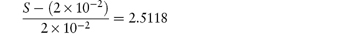
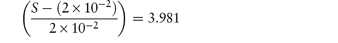
What is the solubility of benzylpenicillin G at a pH sufficiently low to allow only the non-dissociated form of the drug to be present? The pKa of benzylpenicillin G is 2.76 and the solubility of the drug at pH 8.0 is 0.174 mol dm−3. (From Notari RE. Biopharmaceutics and Pharmacokinetics, 2nd edn. New York: Marcel Dekker, 1978.) Answer If only the undissociated form is present at low pH then we need to find S0. This can be obtained from the information given using equation (4.8):
Therefore,
i.e.
Therefore, S0 = 1 × 10⁻⁶ mol dm−3. |


Basic drugs
Basic drugs such as ranitidine are more soluble in acidic solutions, where the ionised form of the drug is predominant. If S0 is the solubility of an undissociated base, RNH2, the Henderson–Hasselbalch expression for the solubility (S) as a function of pH (see Derivation Box 4B) is
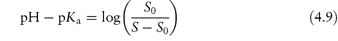
Solubility–pH profiles of a basic drug (chlorpromazine) and an acidic drug (indometacin) and values for the more complex profile of the amphoteric drug oxytetracycline are plotted in Fig. 4.3.
Figure 4.3 Solubility of (a) indometacin, (b) chlorpromazine and (c) oxytetracycline as a function of pH, plotted as logarithm of the solubility.
In general, this approach is valid in dilute ideal solutions for which the solubility of the ionised species is much greater than that of the uncharged species. Despite its widespread use to predict the pH dependence of drug solubility, a study of the accuracy of equation (4.9) in predicting the solubility of a series of cationic drugs as a function of pH in divalent buffer systems mimicking the intestinal fluid highlighted some limitations of this equation and the authors cautioned against its uncritical use.7
|
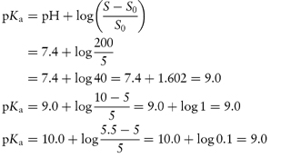
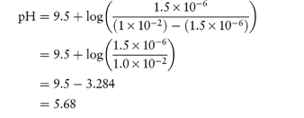
A drug is found to have the following saturation solubilities at room temperature: pH S (μmol dm−3) 7.4 205.0 9.0 10.0 10.0 5.5 12.0 5.0 What type of compound is it likely to be and what is its pKa? Answer As the solubility decreases with increasing pH, the compound is a base. At pH 12 the solubility quoted is likely to be the solubility of the unprotonated species, that is, S0. Using the figures given, we can apply a re-arranged form of equation (4.9) at each of the other pH values:
The drug has a pKa value of 9.0 and is thus likely to be an amine. |

Amphoteric drugs
Several drugs and amino acids, peptides and proteins are amphoteric, displaying both basic and acidic characteristics. Frequently encountered drugs in this category are the sulfonamides and the tetracyclines. If, for simplicity, we were to use a generalised structure for an amphoteric compound

and if the solution equilibrium between the species were written down, we would obtain the following equations relating solubility to pH (see Derivation Box 4C).

at pH values below the isoelectric point, and

at pH values above the isoelectric point.
Table 4.8 gives solubility data for oxytetracycline (XVI) as a function of pH. Oxytetracycline has three pKa values: pKal = 3.27, pKa2 = 7.32 and pKa3 = 9.11, corresponding to the regions 1, 2 and 3 in the structure shown.
Table 4.8 Oxytetracycline: pH dependence of solubility at 20°C
pH | Solubility (g dm−3) |
1.2 | 31.4 |
2 | 4.6 |
3 | 1.4 |
4 | 0.85 |
5 | 0.5 |
6 | 0.7 |
7 | 1.1 |
8 | 28.0 |
9 | 38.6 |
Data from the United States Dispensatory, 25th edn.
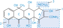
Structure XVI Oxytetracycline
The equations for the solubilities of acidic, basic and zwitterionic drugs (equations 4.8, 4.9, 4.10 and 4.11) can all be used to calculate the pH at which a drug will precipitate from solution of a given concentration (or the concentration at which a drug will reach its maximum solubility at a given pH). This is especially important in determining the maximum allowable levels of a drug in infusion fluids or formulations. Some idea of the range of pH values encountered in common infusion fluids can be seen from the data of Tse et al.8 Typical examples include: Ringer’s solution (pH 7.0), 1 L of Ringer’s solution containing 2 cm3 vitamins (pH 5.5), normal saline (pH 5.4), 5% dextrose in water (pH 4.4), 1 L of 5% dextrose containing 100 mg of thiamine hydrochloride (pH 3.9).
The variation in pH between preparations and within batches of the same infusion fluid (the monograph for Dextrose Infusion BP allows a pH ranging from 3.5 to 5.5) means that the fluids vary considerably in their solvent capacity for weak electrolytes.
Not only is it important to consider the pH of the formulation when deciding on the concentration of drug that can be incorporated, it is equally important to bear in mind possible changes in pH that might occur following administration of the formulation as these might be responsible for drug precipitation from formulations in which the drug concentration is close to the solubility limit. Several examples of the precipitation of drugs in vivo resulting from alteration of pH are considered in Chapter 11 and we will consider here only one example, that of precipitation from eye drop formulations containing amphoteric fluoroquinolone drugs.
Rule of thumb
From the above equations it is seen that, as a rough guide, the solubility of drugs with un-ionised species of low solubility varies by a factor of 10 for each pH unit change. A compilation of the pKa values of drugs is given in Chapter 2 (Table 2.6).
|
Eye drops containing norfloxacin (Chibroxin), ciprofloxacin (Ciloxan) and ofloxacin (Ocuflox) are used for the treatment of external ocular infection and corneal ulcer. Although these products are all formulated as sterile, isotonic, aqueous solutions, preserved with benzalkonium chloride, and all contain 0.3% of the respective fluoroquinolone drug, there have been observations of crystallised corneal deposits only following the clinical use of Ciloxan. The reason for the precipitation of this drug is seen from a consideration of differences in the pH of the formulations (Chibroxin 5.2, Ciloxan 4.5 and Ocuflox 6.4) and also the solubilities of the three fluoroquinolones. As we have seen above, solubility of this class of drug generally exhibits a minimum near physiological pH corresponding to the zwitterionic form of the drug; ciprofloxacin is the least soluble of the commercially available fluoroquinolones, with particularly low solubility near the pH of tears. Figure 4.4 shows the solubility–pH plots for the three drugs up to pH 7.5 (the solubility would, of course, increase at higher pH values as the compounds are amphoteric) and provides an explanation for the precipitation of ciprofloxacin. The pH of the tear film immediately following instillation of the eye drops is determined by the pH of the formulation but returns to the physiological value (pH 6.8) within 15 minutes due to tear turnover and drainage. Superimposed on the solubility profile of each drug in Fig. 4.4 are the total drug concentration and the concentration of drug dissolved in the tear fluid. The decrease of total drug concentration with time is a result of tear turnover and drainage. Following dosing of ofloxacin and norfloxacin (Fig. 4.4a, b), the soluble drug concentration is identical to the total drug concentration at all time points and the tear solution remains clear and particulate-free. Following ciprofloxacin dosing (Fig. 4.4c), however, the soluble drug concentration falls significantly below the total drug concentration at approximately 8 minutes after drug addition (tear pH 6.1). At this pH the drug concentration exceeds the solubility limit, a supersaturated solution is formed and precipitation of ciprofloxacin occurs, producing a milky-white tear solution. At approximately 12 minutes post dose (tear pH 6.6), the soluble ciprofloxacin concentration is reduced to almost half (54%) of the total drug concentration due to continued precipitation. |

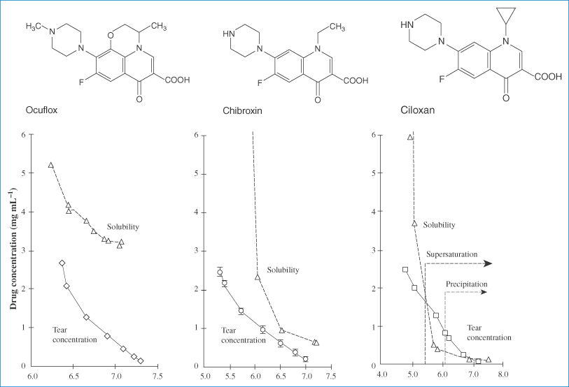
Figure 4.4 Relationship between drug concentration in a tear turnover model (solid lines) and drug solubility (dashed lines) for (a) ofloxacin (Ocuflox); (b) norfloxacin (Chibroxin); and (c) ciprofloxacin (Ciloxan).
Reproduced with permission from Firestone BA et al. Solubility characteristics of three fluoroquinolone ophthalmic solutions in an in vitro tear model. Int J Pharm 1998;164:119. Copyright Elsevier 1998.
|
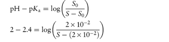
Tryptophan has two pKa values, 2.4 and 9.4, and an isoelectric point of 5.9. Calculate the solubility of tryptophan at pH 2 and at pH 10, given that the solubility of the compound in neutral solutions, S0, is 2 × 10⁻² mol dm−3. Answer At pH 2.0: This pH is below the isoelectric point so we must use equation (4.10):
Rearranging,
That is,
Therefore, S = (5.02 × 10⁻²) + (2 × 10⁻²) = At pH 10 (using equation 4.11):
That is,
Therefore, S = (7.96 × 10⁻²) + (2 × 10⁻²) = 9.96 × 10⁻² mol dm−3. |


| ||||||||||||
Calculate the pH at which the following drugs will precipitate from solution given the information supplied.
The isoelectric point of oxytetracycline HCl is at approx. pH = 5. Answer (a) We use equation (4.9) to calculate the pH above which thioridazine will precipitate:
The concentration of solution is the saturation solubility at the point of precipitation. 0.407% w/v = 1 × 10⁻² mol dm−3 = S. S0 = 1.5 × 10⁻⁶ mol dm−3.
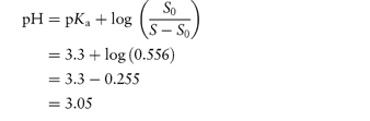
(b) The concentration of solution is 1.4 mg cm−3, which is 1.4 g dm−3. S0 = 0.5 g dm−3. At pH values below the isoelectric point, the pH at which S is the maximum solubility is given by eq (4.10)
At pH values above the isoelectric point, the pH at which S is the maximum value is given by eq (4.11)
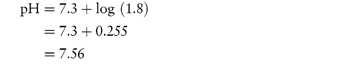
Thus at pH values between 3.05 and 7.56 the solution containing 1.4 mg cm−3 will precipitate. |


4.3 Measurement of solubility
In the traditional method of determining drug solubility, often referred to as the ‘shake flask’ method, the drug is added to a standard buffer solution until saturation occurs, indicated by undissolved excess drug. The pH is remeasured and, if necessary, readjusted with dilute acid or alkali. The flasks are then shaken for a minimum of 24 h and the amount of dissolved drug is determined by a suitable assay of the supernatant solution after filtration. This method is, however, manually intensive and time-consuming, and several alternative procedures have been proposed.
A simple turbidimetric method for the determination of the solubility of acids and bases in buffers of different pH can be used.9 Solutions of the hydrochloride (or other salt) of a basic drug, or the soluble salt of an acidic compound, are prepared in water over a range of concentrations. Portions of each solution are added to buffers of known pH and the turbidity of the solutions is determined in the visible region. Typical results are shown in Fig. 4.5. Below the solubility limit there is no turbidity. As the solubility limit is progressively exceeded, the turbidity rises. The solubility can be determined by extrapolation, as shown in Fig. 4.5. Table 4.9 shows results obtained by this method for some phenothiazines and tricyclic antidepressant compounds. Determination of the solubility of weak electrolytes at several pH values provides one method of obtaining the dissociation constant of the drug substance. For basic drugs,
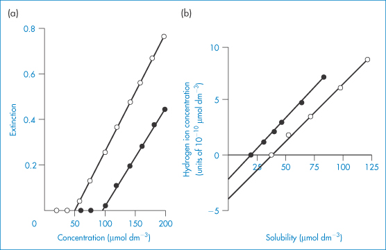
Figure 4.5 (a) Plot of extinction against concentration of amitriptyline hydrochloride at pH 9.78 (○) and pH 9.20. (b) (●) Relationship between hydrogen ion concentration and solubility of pecazine (●) and amitriptyline (○).
Reproduced from Green AL. Ionisation constants and water solubilities of some aminoalkyl phenothiazine tranquillizers and related compounds. J Pharm Pharmacol 1967;19:10–16. Copyright Wiley-VCH Verlag GmbH & Co. KGaA. Reproduced with permission.
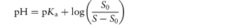
Table 4.9 Water solubilities and pKa values of aminoalkylphenothiazines and related compounds
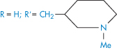
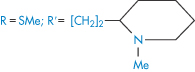
Structure | Approved name | pKa, solubility method | pKa, Chatten–Harrisa | Solubility (μ mol dm−3) | Calculated relative solubility at pH 7.4 |
R═H;R′═CH2CH(Me) • NMe2 | Promethazine | 9.1 | 9.1 | 55 | 4.5 |
R═H;R′═[CH2]3 • NMe2 | Promazine | 9.4 | – | 50 | 8.0 |
R═Cl; R′═[CH2]3 • NMe2 | Chlorpromazine | 9.3 | 9.2 | 8 | 1.0 |
R═CF3; R′═[CH2]3 • NMe2 | Triflupromazine | 9.2 | 9.4 | 5 | 0.4 |
| Pecazine | 9.7 | – | 18 | 5.0 |
| Thioridazine | 9.5 | 9.2 | 1.5 | 0.3 |
Reproduced from Green AL. Ionisation constants and water solubilities of some aminoalkyl phenothiazine tranquillizers and related compounds. J Pharm Pharmacol 1967;19:10–16. Copyright Wiley-VCH Verlag GmbH & Co. KGaA. Reproduced with permission.
aData from Chatten LG, Harris LE. Anal Chem 1962;34:1495.
S0, the solubility of the undissociated species (base), is determined at high pH, and S is determined at several different lower pH values. A plot of log[S0/(S − S0)] versus pH will have the pKa as the intercept on the pH axis.
Alternatively, S may be plotted against [H+], as in Fig. 4.5b. The dissociation of a basic drug in water may be written as (see Derivation Box 4B)
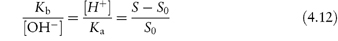
which can be rearranged to
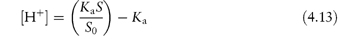
Plotting data as in Fig. 4.5b yields S0 when the line crosses the x-axis as [H+] = 0 (and S = S0). The intercept on the y-axis gives −Ka and the slope of the line is Ka/S0.
4.4 The solubility parameter
Regular solution theory characterises non-polar solvents in terms of solubility parameter, δ1, which is defined as
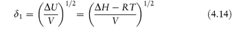
where ΔU is the molar energy and ΔH is the molar heat of vaporisation of the solvent. ΔH is determined by calorimetry at temperatures below the boiling point at constant volume. V is the molar volume of the solvent. The solubility parameter is thus a measure of the intermolecular forces within the solvent and gives us information on the ability of the liquid to act as a solvent. Table 4.10 gives the solubility parameters of some common solvents calculated using equation (4.14).
Table 4.10 Solubility parameters of common solvents
Solvent | δ1 (cal1/2 cm−3/2)a |
Methanol | 14.50 |
Ethanol | 12.74 |
1-Propanol | 11.94 |
2-Propanol | 11.56 |
1-Butanol | 11.40 |
1-Octanol | 10.24 |
Ethyl acetate | 8.58 |
Isoamyl acetate | 8.07 |
Hexane | 7.30 |
Hexadecane | 8 |
Carbon disulfide | 10 |
Membrane (erythrocytes) | 10.3 ± 0.40 |
Cyclohexane | 8.2 |
Benzene | 9.2 |
aThe solubility parameter is commonly expressed in hildebrand units:
1 hildebrand unit = 1 (cal cm−3)1/2.
1 cal = 4.18 J.
ΔU/V is the liquid’s cohesive energy density, a measure of the attraction of a molecule from its own liquid, which is the energy required to remove it from the liquid and is equal to the energy of vaporisation per unit volume. Because cavities have to be formed in a solvent, by separating other solvent molecules, to accommodate solute molecules (as discussed earlier) the solubility parameter δ1 enables predictions of solubility to be made in a semiquantitative manner, especially in relation to the solubility parameter of the solute, δ2.
By itself the solubility parameter can explain the behaviour of only a relatively small group of solvents – those with little or no polarity and those unable to participate in hydrogen-bonding interactions. The difference between the solubility parameters expressed as (δ1 − δ2) will give an indication of solubility relationships.
For solid solutes a hypothetical value of δ2 can be calculated from (U/V)1/2, where U is in this case the lattice energy of the crystal. In a study of the solubility of ion pairs in organic solvents it has been found that the logarithm of the solubility (log S) correlates well with (δ1 − δ2)2.
4.4.1 Solubility parameters and biological processes
The solubility of small molecules in biological membranes is of importance from pharmacological, physiological and toxicological viewpoints. Biological membranes are not simple solvents – the bilayer has an interior core of hydrocarbon chains about 2.5–3.5 nm thick – and therefore one would not expect simple solution theory to hold. Regular solution theory has been applied to biomembranes to obtain a value of δ1 for a membrane.10 From experimental solubility data for anaesthetic gases in erythrocyte ghosts, mean empirical solubility parameters of 10.3 ± 0.40 for the whole membrane and 8.7 ± 1.03 for membrane lipid were calculated. The values compare with solubility parameters of 7.3 for hexane and 8.0 for hexadecane. The value for the whole membrane (10.3) is very close to the solubility parameter of 1-octanol (10.2), a solvent that is used widely in partition coefficient work to simulate biological lipid phases.
Solubility parameters of drugs (δ2) have also been correlated with membrane absorption rates in model systems. A reasonable relationship was obtained between δ2 and a logarithmic absorption term, thus providing one predictive index of absorption. Scott11 has said of solubility parameters and equations employing them that ‘the theory offers a useful initial approach to a very wide area of solutions. Like a small-scale map for a very broad long-distance view of a sub-continent they are unlikely to prove highly accurate when a small area is examined carefully, but they are equally unlikely to prove completely absurd.’
4.5 Solubility in mixed solvents: use of cosolvents
The device of using mixed solvents (cosolvents) is resorted to when drug solubility in one solvent is limited or perhaps when the stability characteristics of soluble salts forbid the use of single solvents. Cosolvent use is widespread during the screening of new molecular entities as potential drug candidates where large numbers of molecules need to be brought into solution to be tested for biological activity. For such testing in tissue culture or in experimental animals it is important that the drug does not precipitate in the system under study, as this will affect the apparent activity. Common water-miscible solvents used in pharmaceutical formulations include glycerol, propylene glycol, ethyl alcohol and polyoxyethylene glycols, particularly polyoxyethylene glycol 400 (PEG 400). Ethanol is frequently combined with propylene glycol in cosolvent mixtures, for example phenobarbital is solubilised in a cosolvent mixture of 68–75% propylene glycol and 10% ethanol; pentobarbital sodium, phenytoin sodium and digoxin are all solubilised in solutions with 40% propylene glycol and 10% ethanol. Cosolvent formulations often contain several organic cosolvents; for example, the sparingly water-soluble antineoplastic agent etoposide is solubilised in a cosolvent mixture of PEG 400, glycerin and water; digoxin is solubilised in a cosolvent mixture of propylene glycol, PEG 400 and ethanol; parenteral solutions of diazepam contain propylene glycol, ethanol and benzyl alcohol. As can be imagined, the addition of another component complicates any system and explanations of the often complex solubility patterns are not easy. Toxicity considerations are, of course, a constraint on the choice of solvent for products for administration by any route.
The range of solubilty of phenobarbital in common mixed solvents is seen from the data of Krause et al.12 Phenobarbital dissolves up to 0.12% w/v in water at 25°C. Glycerol, even in high concentrations, does not significantly increase the solubility of the drug (the solubility increases to only 1% w/v in 100% glycerol). Ethanol is a much more efficient cosolvent than glycerol as it is less polar. Phenobarbital solubility reaches a maximum of 13.4% w/v at 90% ethanol in ethanol–water mixtures, and 16% w/v at 80% ethanol in ethanol–glycerol mixtures. Adding an organic cosolvent to water makes the solvating environment less polar, resulting in a more favourable mixing (solvation) of a hydrophobic solute in the liquid phase. One key aspect of drug solubilisation with the aid of cosolvents is to create a solvent mixture that closely matches the polarity of the hydrophobic solute. In general, the more hydrophobic the solute, the greater the solubilising effect produced by an organic cosolvent that is less polar than water.
A proposed model for prediction of the solubility, Sm, of organic compounds in mixed solvents composed of water and an organic cosolvent, the log-linear cosolvency model, assumes that the solubility in the water–cosolvent mixture, Sm, increases logarithmically with a linear increase in the fraction of organic solvent according to

where fc and fw are the volume-fraction concentrations of the organic cosolvent and water, respectively, and Sc and Sw, are the solubilities in pure cosolvent and water, respectively. The model is based on the assumption that the free energy of solution of the mixture corresponds to the (volume-fraction) weighted average of the free energy of solution in the pure solvent components.
Rearranging equation (4.15) and noting that fw = 1 – fc gives

where σ = log (Sc/Sw) or, more correctly, log (γw/γc) where γw and γc are the activity coefficients of the solute in water and pure organic solvent, respectively. The model therefore predicts a linear relationship between the logarithm of the solubility in the mixed solvent and the volume fraction of the cosolvent in the mixed solvent. The gradient of the plot is σ and the intercept is the logarithm of the solubility of the drug in water.
The σ term is often referred to as the cosolvency power, since it provides a measure of the inherent ability of the particular cosolvent to solubilise the solute in relation to its solubility in water. The σ parameter has the properties of a hypothetical partition coefficient. For example, for a given organic solvent, the σ parameter of different solutes is linearly related to their octanol–water partition coefficient, such that σ estimates can be made from the σ values of other solutes in the same cosolvent.
The model assumes that the solute–water and solute–cosolvent interactions are present in the water–cosolvent mixture in direct proportion to the respective concentration of each of the solvents in the solvent blend. The model also assumes that no additional interactions exist in the solvent mixture apart from these. The polarity match predicted by the log-linear model has been shown to apply when polar cosolvents such as aliphatic alcohols (methanol, ethanol, propanol) are used but is less predictable with less polar cosolvents such as tetraglycol, Labrasol and 1-methyl-2-pyrrolidone, because of cosolvent–water interactions.13
The situation becomes more complex when additives are included in the formulation as these will influence solute–solvent interfacial energies or dissociation of electrolytes through changes in dielectric constant. A reduction in ionisation through a decrease in dielectric constant will favour decreased solubility, but this effect may be counterbalanced by the greater affinity of the undissociated species in the presence of the cosolvent.
Problems which may arise from precipitation of poorly water-soluble drugs during the administration of mixed-solvent systems are discussed in the following clinical point and in more detail in Chapter 11 (section 11.2).
Room-temperature ionic liquids
An interesting class of solvents with potential application for the solubilisation of poorly water-soluble drugs are the room-temperature ionic liquids (RTILs).14 These are organic salts comprising a relatively large asymmetric organic cation (e.g. alkyl pyridinium and dialkyl imidazolium ions) combined with an inorganic or organic anion (e.g. halide, hexafluorophosphate and tetrafluoroborate) which, as the name implies, are liquid at ambient temperature. Their versatility as solvents arises from the wide range of possible combinations of the constituent anions and cations providing a correspondingly wide variation of acidity, basicity, hydrophilicity/hydrophobicity and water miscibility. Typical examples are given in Structure XVII which shows RTILs based on 1-alkyl-3-methylimidazolium cations combined with PF6–, Cl–, BF4– and Br– anions. The ability of some of these RTILs to act as solvents for the poorly water-soluble drugs albendazole and danazol is shown in Table 4.11 from which it is seen that the longer the alkyl chain of the cation (i.e. the greater the hydrophobicity), the greater is the solubility enhancement.
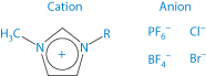
Structure XVII Room-temperature ionic liquids based on 1-alkyl-3-methylimidazolium cations
The miscibility of RTILs with water can be improved by inclusion of a second RTIL enabling their application as cosolvents in aqueous systems. For example, the solubility of albendazole in mixtures of water/C4H9imidazolium PF6–/ C6H13imidazolium Cl– at a 1/1/1 molar ratio was 7.95 mmol/L compared to a water solubility of 0.002 mmol/L.
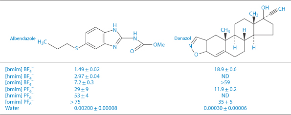
Table 4.11 Solubility (mmol/L, mean ± SD, n = 3) of two model drugs in room-temperature ionic liquids based on the 1-alkyl-3-methylimidazolium cations (XVII) with alkyl chain lengths: R = C4H9 [bmim]; C6H13 [hmim]; C8H17 [omim]. ND = not determined.
Reproduced from Mizuuchi H et al. Room temperature ionic liquids and their mixtures: potential pharmaceutical solvents. Eur J Pharm Sci 2008;33:326–331.
|
A potential problem associated with the administration of mixed-solvent formulations of poorly water-soluble drugs is drug precipitation when these preparations are added to an aqueous solution such as blood plasma. For example, precipitation of the relatively water-insoluble diazepam has been reported when formulations of this drug in a mixed-solvent solution containing propylene glycol (40%) and alcohol (10%) are administered by injection using an intravenous (IV) infusion set, rather than directly into the vein of the patient, as instructed by the supplier. Precipitation occurs because of changes in the proportions of the solvents on dilution with plasma in the infusion set; we discuss this problem in more detail in Chapter 11 (section 11.2). Precipitation of a poorly water-soluble drug during IV injection may also be a consequence of a rapid infusion rate or abnormally slow venous flow rate, both of which result in unfavourable changes in solvent composition. The critical parameters that determine whether a drug will precipitate during IV injection are its solubility in plasma, the drug dose and the plasma flow rate in the vein. The maximum infusion rate (mg min−1) is the product of the plasma solubility (mg cm−3) and the venous flow rate (normally between 40 and 60 cm3 min−1). Example 4.6 shows the calculation of minimum injection times for a poorly water-soluble drug and illustrates the influence of the rate of venous flow on the time required to prevent precipitation of drug in the plasma. Note that in this calculation it is assumed that the injected solution mixes instantaneously with the plasma; in practice longer injection times should be used to ensure safety. |

|
What is the minimum time required for the IV injection of a 20 mg dose of a poorly water-soluble drug (solubility in plasma = 0.60 mg cm−3) to ensure that precipitation does not occur? Assume a venous flow rate of (a) 60 cm3 min−1and (b) 40 cm3 min−1. Answer (a) Maximum infusion rate = plasma solubility × venous flow rate:
Therefore, a 20 mg dose should be injected over a period of at least 33 seconds to avoid drug precipitation. (b) Maximum infusion rate = 0.60 × 40 = 24.0 mg min−1. Therefore, at least 50 seconds should be allowed for injection at this venous flow rate. |


4.6 Cyclodextrins as solubilising agents
Solubilisation by surface-active agents is discussed in Chapter 5. Alternatives to micellar solubilisation (or solubilisation in vesicles) include the use of the cyclodextrin (CD) family. When the first edition of this book was published in 1981 (and a diagram of a CD–drug complex was used to adorn the cover), the use of CDs was in its infancy. Attention was then focused around α-, β- and γ-CDs, but a veritable industry has grown up with an array of derivatives that can lend useful new properties to the complexes they form. For example, 10% of the CD derivative Encapsin HPB (hydroxypropyl-β-cyclodextrin) can enhance the aqueous solubility of betamethasone 118 times, of diazepam 21 times and of ibuprofen 55 times. The solubilising capacities of a range of CDs and their derivatives have been reviewed.15 An idea of the extent to which natural CDs and their derivatives are currently included in marked pharmaceutical products is seen from Table 4.12, which details just some of the estimated 35 different commercial formulations. This topic has been comprehensively reviewed by Kurkov and Loftsson.16
Table 4.12 Marketed pharmaceutical products which include natural cyclodextrins (αCD, and βCD) and the cyclodextrin derivatives 2-hydroxypropyl-β-cyclodextrin (HPβCD), sulfobutylether β-cyclodextrin sodium salt (SBEβCD) and 2-hydroxypropyl-γ-cyclodextrin (HP γCD)
Drug/cyclodextrin | Therapeutic usage | Formulation | Trade name |
αCD |
|
|
|
AlprostadilI | Treatment of erectile dysfunction | Intracavernous solution | CaverJect Dual |
βCO |
|
|
|
Cetirzine | Antibacterial agent | Chewing tablets | Cetrizin |
Dexamethasone | Anti-Inflammatory steroid | Ointment, tablets | Glymesason |
Nicotine | Nicotine replacement product | Sublingual tablets | Nicorette |
Nimesulide | Non-steroidal anti-inflammatory drug | Tablets | Nimedex |
Piroxicam | Non-steroidal anti-inflammatory drug | Tablets, suppository | Brexin |
HPβCD |
|
|
|
Indomethacin | Non-steroidal anti-inflammatory drug | Eye drop solution | Indocid |
Itraconazole | Antifungal agent | Oral and IV solutions | Sporanox |
Mitomycin | Anticancer agent | IV infusion | MitoExtra |
SBEβCD |
|
|
|
Aripiprazole | Antipsychotic drug | IM solution | Abllify |
Maropitant | Anti-emetic drug (motion sickness in dogs) | Parenteral solution | Cerenia |
Voriconazole | Antifungal agent | IV solution | Vfend |
Ziprasidone mesylate | Antipsychotic drug | IM solution | Geodon |
HPyCD |
|
|
|
Diclofenac sodium salt | Non-steroidal anti-Inflammatory drug | Eye drop solution | Voltaren Ophtha |
Tc-99 Teoboroxime | Diagnostic aid, cardiac imaging | IV solution | CardioTec |
Reproduced from Loftsson T, Brewster ME. Pharmaceutical applications of cyclodextrins. 1. Drug solubilization and stabilization. J Pharm Sci 1996;85:1017–1025. Copyright Wiley-VCH Verlag GmbH & Co. KGaA. Reproduced with permission.
CDs are enzymatically modified starches. Their glucopyranose units form a ring: α-CD a ring of 6 units; β-CD a ring of 7 units; and γ-CD a ring of 8 units (Table 4.13; Fig. 4.6). The ‘ring’ is cylindrical, the outer surface being hydrophilic and the internal surface of the cavity being non-polar. Appropriately sized lipophilic molecules can be accommodated wholly or partially in the complex, in which the host–guest ratio is usually 1 : 1 (Fig. 4.7), although other stoichiometries are possible, one, two or three CD molecules complexing with one or more drug molecules. The dissolution–dissociation–crystallisation process that can occur on dissolution is illustrated in Fig. 4.8.
Table 4.13 Properties of α, β and γ cyclodextrins
Property | Alpha (α) | Beta (β) | Gamma (γ) |
Molecular weight | 973 | 1135 | 1297 |
Glucose monomers | 6 | 7 | 8 |
Internal cavity diameters (nm) | 0.5 | 0.6 | 0.8 |
Water solubility (g 100 cm–3; 25°C) | 14.2 | 1.85 | 23.2 |
Surface tension (mN m−1) | 71 | 71 | 71 |
Melting range (°C) | 255–260 | 255–260 | 240–245 |
Water of crystallisation (no. of molecules) | 10.2 | 13–15 | 8–18 |
Water in cavity (no. of molecules) | 6 | 11 | 17 |
Reproduced with permission from Brewster ME et al. Development of a non-surfactant formulation for alfaxalone through the use of chemically-modified cyclodextrins. J Parenter Sci Technol 1989;43:262.
Figure 4.6 Structures of the α-, β- and γ-cyclodextrins.
Reproduced from Szejtli J. Pharm Tech Int 1991;3(2):15.
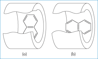
Figure 4.7 Two models of a complex of cyclodextrin with a lipophilic guest compound: (a) equatorial inclusion, (b) axial inclusion.
Reproduced with permission from Harata K, Uedaira H. Bull Chem Soc Jpn 1975;48:375.
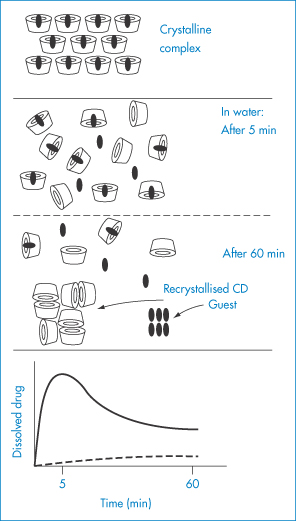
Figure 4.8 Schematic representation of the dissolution–dissociation–recrystallisation process of a cyclodextrin complex with a poorly soluble guest. The complex rapidly dissolves, and a metastable oversaturated solution is obtained. The anomalously high level of dissolved guest drops back but remains higher than the level that can be obtained with non-complexed drug. Solid curve = complexed drug; broken curve = non-complexed drug.
Redrawn after Szejtli J. Pharm Tech Int 1991;3(2):15.
Not all CDs are free of adverse effects; di-O-methyl β-CD, for example, has a strong affinity for cholesterol and is haemolytic. It is also one of the best solubilisers technically.
The CDs have obvious uses in parenteral formulations, including use as components of vehicles for peptides and other biologicals (ovine growth hormone, interleukin-2 and insulin). A special use of one γ-CD derivative, sugammadex, is discussed in Chapter 11 (section 11.6.1). Because it tightly binds the general anaesthetic rocuronium when injected IV it reverses its action and thus shortens the duration of anaesthesia at will.
Calixarenes
Research continues into other agents, apart from surfactants (which are discussed in Chapter 5), that can enhance the solubility of drugs. The calixarenes are another type of host, existing in a ‘cup shape’ in a rigid conformation. The 4-sulfonic calix[n]arenes can form host–guest-type interactions with drugs such as nifedipine, a poorly water-soluble agent,17 seen in Fig. 4.9.
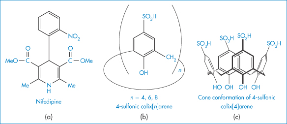
Figure 4.9 Molecular structures of (a) nifedipine and (b) 4-sulfonic calix[n]arenes. As n increases (4, 6, 8) the cavity size (see (c)) increases from 0.3 nm, through 0.76 nm to 1.16 nm. The solubility increase for nifedipine is greatest with calix[8]arene, being nearly 250% at a concentration of 0.008 mol dm−3 and pH of 5.
Reproduced with permission from Yang W, de Villiers MM. The solubilization of the poorly water soluble drug nifedipine by water soluble 4-sulphonic calix[n]arenes. Eur J Pharm Biopharm 2004;58:629–636. Copyright Elsevier 2004.
4.7 Solubility problems in formulation
4.7.1 Mixtures of acidic and basic compounds
Sometimes a combination formulation requires the admixture of acidic and basic drugs. One example (Septrin infusion) is discussed here.
Because sulfamethoxazole (XVIII) is a weakly acidic substance and trimethoprim (XIX) is a weakly basic one, for optimal solubility basic and acidic solutions, respectively, are required. In consequence, in an ordinary aqueous solution sulfamethoxazole and trimethoprim demonstrate a high degree of incompatibility and mutual precipitation occurs on mixing. To optimise mutual dissolution, an aqueous solution that includes 40% propylene glycol is used in the formulation of the infusion. This solution, which has a pH between 9.5 and 11.0, allows adequate amounts of both substances to coexist in solution to give the correct ratio of concentration for antibacterial action. On dilution, the infusion becomes less stable and at the recommended 1 in 25 dilution stability is about 7 h. Owing to incompatibility of the two constituents, their degrees of solubility are sensitive to changes in ionic composition, pH and any drug additives. If there is imbalance in pH or ionic composition, then precipitation of one or other of the components may well occur.
Structure XVIII Sulfamethoxazole, pKa = 6.03
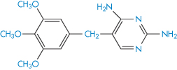
Structure XIX Trimethoprim, pKa = 7.05
4.7.2 Choice of drug salt to optimise solubility
The choice of a particular salt of a drug for use in formulations may depend on several factors. The solubility of the drug in aqueous media may be markedly dependent on the salt form. The chemical stability rather than the solubility may be a criterion and in many cases this is dependent on the choice of salt, sometimes through a pH effect. Deliberate choice of an insoluble form for use in suspensions is an obvious ploy; the formation of water-soluble entities from poorly soluble acids or bases by the use of hydrophilic counterions is frequently attempted to produce injectable solutions of a drug. Table 4.14 gives some indication of the range of solubilities that can be obtained through the use of different salt forms, in this case of an experimental antimalarial drug (XX).
Table 4.14 Solubilities of salts of an antimalarial drug (XX)
Salt | Melting point (°C)a | Solubility (mg cm−3) | Saturated solution pH |
Free base | 215 | 7–8 | – |
Hydrochloride | 331 | 32–15 | 5.8 |
dl-Lactate | 172 (dec) | 1800 | 3.8 |
l-Lactate | 193 (dec) | 900 | – |
2-Hydroxy-1-sulfonate | 250 (dec) | 620 | 2.4 |
Methanesulfonate | 290 (dec) | 300 | 5.1 |
Sulfate | 270 (dec) | 20 | – |
a(dec) = with decomposition.
Reproduced from Agharkar S et al. Enhancement of solubility of drug salts by hydrophilic counterions: properties of organic salts of an antimalarial drug. J Pharm Sci 1976;65:747. Copyright Wiley-VCH Verlag GmbH & Co. KGaA. Reproduced with permission.
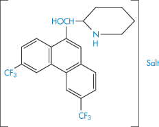
Structure XX Compound used in Table 4.14
The large hydrophobic compound XX, even as its hydrochloride salt, is poorly soluble and this is presumably the reason for its poor oral bioavailability. Similar conclusions were drawn several years ago for novobiocin. The acid salt administered to dogs at 12.5 mg kg−1 was not absorbed, but the monosodium salt, which is about 300 times as soluble in water, produced plasma levels of 22 μg cm−3 after 3 h. Unfortunately, the sodium salt is unstable in solution. An amorphous form of the acid produced even higher levels of drug than the sodium salt, illustrating the fact that choice of salt and crystalline form of a drug substance may be of critical importance.
Some of the solubility differences obviously arise from differences in the pH of the salt solutions, which in the case of compound XX ranged from 2.4 to 5.8 pH units. This is not atypical. The pH of solutions of salts of a 3-oxyl-1,4-benzodiazepine derivative at 5 mg cm−3 ranged from 2.3 for its dihydrochloride, to 4.3 for the maleate, and to 4.8 for the methanesulfonate.
Further examples of the solubility range in drug salts and derivatives are shown in Table 4.15. The increase in the solubility on the formation of the hydrochloride is readily attributable in the case of tetracycline to a lowering of the solution pH by the hydrochloride. The common ion effect (see section 4.2.3) can, however, produce an unexpected trend in the solubilities and dissolution rates (since these are proportional to the solubility in the diffusion layer at the surface of the solid) of bases in the presence of high concentrations of hydrochloric acid.18 Increase in Cl− concentrations will cause the equilibrium between solid (s) and solution (aq) forms

to be pushed to the left-hand side, with a resultant decrease in solubility. The solubility of XX as the hydrochloride decreases from 24 × 10−5 mol dm−3 in 1.3 mmol dm−3 chloride ion, to 3 × 10⁻⁵ mol dm−3 in 40 mmol dm−3 chloride ion concentration. It should be noted that the stomach contents are rich in chloride ions. The common ion effect will be apparent in many infusion fluids to which drugs may be added, and therefore the effect of pH as well as electrolyte concentrations must be considered.
Table 4.15 Aqueous solubilities of tetracycline, erythromycin and chlorhexidine salts
Compound | Solubility in water (mg cm−3) |
Tetracycline | 1.7 |
Tetracycline hydrochloride | 10.9 |
Tetracycline phosphate | 15.9 |
Erythromycin | 2.1 |
Erythromycin estolatea | 0.16 |
Erythromycin stearate | 0.33 |
Erythromycin lactobionate | 20 |
Chlorhexidine | 0.08 |
Chlorhexidine dihydrochloride | 0.60 |
Chlorhexidine digluconate | >700 |
aLauryl sulfate ester of erythromycin propionate
Consideration of Table 4.15 suggests that the hydrochloride salts of tetracyclines are always more readily dissolved than the base. The situation is more complex than at first appears, however. In dilute HCl at pH 1.2, the free base dissolves more than the hydrochloride, probably owing to the differences in crystallinity. The amount of compound derived from the base in solution decreases with time as the drug is converted to the hydrochloride. At pH 1.6 the rate of solution of the two forms is identical, and at pH 2.1 the hydrochloride has a higher solubility owing to its effect on local pH around the dissolving particles.
Erythromycin (XXI) is labile at pH values below pH 4, and hence is unstable in the stomach contents. Erythromycin stearate (the salt of the tertiary aliphatic amine and stearic acid), being less soluble, is not as susceptible to degradation. The salt dissociates in the intestine to yield the free base, which is absorbed. There are differences in the absorption behaviour of the erythromycin salts and differences in toxicity, which may be related to their aqueous solubilities. Erythromycin ethylsuccinate was originally developed for paediatric use because its low water solubility and relative tastelessness were suited to paediatric formulations. The soluble lactobionate is used in IV infusions.
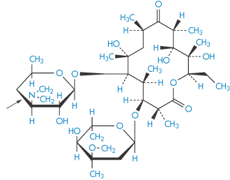
Structure XXI Erythromycin
4.7.3 Drug solubility and biological activity
There should be a broad correlation between aqueous solubility and indices of biological activity. On the one hand, as drug solubility in aqueous media is inversely related to the solubility of the agent in biological lipid phases, there will be some relationship between pharmacodynamic activity and drug solubility. On the other, we should expect that drug or drug salt solubility might influence the absorption phase; drugs of very low aqueous solubility will dissolve slowly in the gastrointestinal tract, and in many cases the rate of dissolution is the rate-controlling step in absorption.
With drugs of low aqueous solubility such as digoxin, chlorpropamide, indometacin, griseofulvin and many steroids, the physical properties of the drug can influence biological properties. At early stages in a drug’s development, pharmacological and toxicological tests are frequently carried out on extemporaneously prepared suspensions whose physical characteristics are not always well defined. This is not good practice as the toxicity of some drugs given by gavage to rats is dependent on the drug species used19 (Table 4.16). This has been shown to be true with polymorphic forms of the same drug, but in the cases discussed in Table 4.16 different salts of the drugs were used.
Table 4.16 The effect of solubility in water on the toxicity of drugs given by gavage to albino rats
Drug | Salt | Solubility | LD50 ± SEM |
Benzylpenicillin | Ammonium | <20 mg cm−3 | 8.4 ± 0.13 |
Benzylpenicillin | Potassium | >20 mg cm−3 | 6.7 ± 0.1 |
Iron | Free metal | Insoluble | 98.6 ± 26.7 |
Iron | Ferrous sulfate | Soluble | 0.78 |
Spiramycin | Free base | Poorly soluble | 9.4 ± 0.8 |
Spiramycin | Adipate | Soluble | 4.9 ± 0.2 |
Modified from Boyd E. Predictive Toxicometrics. Bristol: Scientechnica; 1972.
There are other examples in which aqueous solubility acts as a rough and ready guide to absorption characteristics. The least soluble of the cardiotonic glycosides (digitoxin, digoxin and ouabain), being the most lipid soluble, are best absorbed. But because of the lipophilicity of digitoxin and digoxin, the rate-limiting step is the rate of solution, which is influenced directly by the solubility of the compounds.
High-molecular-weight quaternary salts such as bephenium hydroxynaphthoate (XXII) and pyrvinium embonate (XXIII), being quaternary, have low lipid solubility but also have low aqueous solubility. They are virtually unabsorbed from the gut and indeed are used in the treatment of worm infestation of the lower bowel.
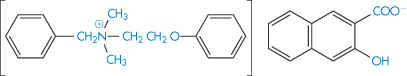
Structure XXII Bephenium hydroxynaphthoate
Structure XXIII Pyrvinium embonate
|
|

4.8 Partitioning
Here we discuss the topic of partitioning of a drug or solute between two immiscible phases. One phase might be blood or water and the other a biomembrane, or an oil or a plastic. As many processes (not least the absorption process) depend on the movement of molecules from one phase to another, it is vital that this topic is mastered. Here we will learn of the simple concepts of the partitioning of drugs and the calculation of partition coefficient (P) of the un-ionised form of the solute (and its logarithm, log P), as well as the use of the log P concept in determining the relative activities or toxicities of drugs from a knowledge of log P between an oil, most commonly octanol, and water. Where P cannot be measured, calculations of log P can be accomplished.20, 21 An outline of the methods available is given here.
Whether in formulations containing more than one phase or in the body, drugs move from one liquid phase to another in ways that depend on their relative concentrations (or chemical potentials) and their affinities for each phase. So a drug will move from the blood into extravascular tissues if it has the appropriate affinity for the cell membrane and the non-blood phase.
The movement of molecules from one phase to another is called partitioning. Examples of the process include:
- drugs partitioning between aqueous phases and lipid biophases
- preservative molecules in emulsions partitioning between the aqueous and oil phases
- antibiotics partitioning into microorganisms
- drugs and preservative molecules partitioning into the plastic of containers or giving sets.
Plasticisers will sometimes partition from plastic containers into formulations. It is, therefore, important that the process can be quantified and understood.
4.8.1 The partition coefficient
If two immiscible phases are placed in contact, one containing a solute soluble to some extent in both phases, the solute will distribute itself so that when equilibrium is attained no further net transfer of solute takes place, as then the chemical potential of the solute in one phase is equal to its chemical potential in the other phase. If we think of an aqueous (w) and an organic (o) phase, we can write, according to equations (2.28) and (2.30),

Rearranging equation (4.17) we obtain
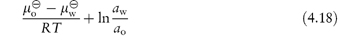
The term on the left-hand side of equation (4.18) is constant at a given temperature and pressure, so it follows that aw/ao = constant and, of course ao/aw = constant. These constants are the partition coefficients or distribution coefficients, P. If the solute forms an ideal solution in both solvents, activities can be replaced by concentration, so that
P is therefore a measure of the relative affinities of the solute for an aqueous and a non-aqueous or lipid phase. Unless otherwise stated, P is calculated according to the convention in equation (4.19), where the concentration in the non-aqueous (oily) phase is divided by the concentration in the aqueous phase. The higher the value of P, the greater is the lipid solubility of the solute.
It has been shown for several systems that the partition coefficient can be approximated by the solubility of the agent in the organic phase divided by its solubility in the aqueous phase, a useful starting point for estimating relative affinities.
As early as 1891, Nernst stressed the fact that the partition coefficient as a function of concentration would be constant only if a single molecular species were involved. In some systems the association of the solute in one of the solvents complicates the calculation of partition coefficient; a simple example of the treatment of the partitioning of a dimerising compound gives the following equation for the partition coefficient (see Derivation Box 4D).
Table 4.17 illustrates the use of equations (4.19) and (4.20). Being weak electrolytes, many drugs will ionise in at least one phase, usually the aqueous phase. The partitioning of the drug between the organic and water phases depends on the ionic state of the drug and, as we have seen in section 2.5, this is determined by its pKa and the pH of the aqueous phase. The partition coefficient refers to the distribution of one species, in this case the un-ionised drug, whereas the assay method will usually determine both the ionised and un-ionised drug in the aqueous phase. Because ionised species cannot, in general, partition into organic hydrophobic solvents, the ratio of drug concentrations in organic and aqueous phases determined from assay data will yield an apparent partition coefficient, Papp, which will vary with pH, rather than the true partition coefficient P. The relationship between the true thermodynamic P and Papp is given by the following equations, which have been derived in Derivation Box 4D:
For acids:
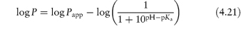
For bases:
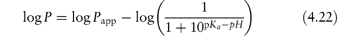
Table 4.17 Distribution of two acids between immiscible phases at 25°C
C1 (mol dm−3)a | C2 (mol dm−3)b | C2/C1 |
|
Succinic acid | |||
0.191 | 0.0248 | 0.130 |
|
0.370 | 0.0488 | 0.132 |
|
0.547 | 0.0736 | 0.135 |
|
0.749 | 0.1010 | 0.135 |
|
Benzoic acid | |||
4.88 × 10⁻³ | 3.64 × 10⁻² | 7.46 | 39.06 |
8.00 × 10⁻³ | 8.59 × 10⁻² | 10.75 | 36.63 |
16.00 × 10⁻³ | 33.8 × 10⁻² | 21.13 | 36.36 |
23.7 × 10⁻³ | 75.3 × 10⁻² | 31.77 | 36.63 |

Reproduced with permission from Glasstone S, Lewis D, Elements of Physical Chemistry, 2nd edn. London: Macmillan; 1964.
aAqueous-phase concentration.
bNon-aqueous-phase concentration (succinic acid in ether; benzoic acid in benzene).
4.8.2 Free energies of transfer
The standard free energy of transfer of a solute between two phases is given by

In a homologous series, P can be measured and the increase in its value observed for each substituent group (for example, ‒CH2‒). As the chain length of non-polar aliphatic compounds increases, it has been found that P increases by a factor of 2–4 per methylene group. The substituent contributions to P are additive, so a substituent constant, πX, may be defined as

where PX is the partition coefficient of the derivative of the parent compound whose partition coefficient is PH and πX is the logarithm of the partition coefficient of the function X. For example, πCl can be obtained by subtracting log Pbenzene from log Pchlorobenzene.
4.8.3 Octanol as a non-aqueous phase
Octanol is often used as the non-aqueous phase in experiments to measure the partition coefficient of drugs. Its polarity means that water is solubilised to some extent in the octanol phase and thus partitioning is more complex than with an anhydrous solvent, but perhaps its usefulness stems from the fact that biological membranes are also not simple anhydrous lipid phases. While octanol is favoured, other alcohols have also been used. For example, isobutanol has been used to show that the binding of many drugs to serum protein is determined by the hydrophobicity or lipophilicity of the drug, following the relationship

where K is an equilibrium constant measuring the binding of solute to protein. Transfer of a hydrophobic drug from an aqueous phase to a protein is, of course, a type of partitioning.
The correlation of lipophilicity and biological activity usually involves equations of the type
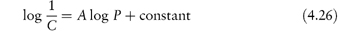
where C is the concentration required to produce a given pharmacological response.
4.9 Biological activity and partition coefficients: thermodynamic activity and Ferguson’s principle
As the site of action of many biologically active species is in lipid components such as membranes, correlations between partition coefficients and biological activity were found early on by investigators of structure–action relationships. For example, a wide range of simple organic compounds can exert qualitatively identical depressant actions (narcosis) on many simple organisms. Lack of any chemical specificity in the compounds tested led to the suggestion that physical, rather than chemical, properties governed the activity of the compounds. Early work by Meyer (in 1899) and Overton (in 1895) related narcotic potency to the oil/water partition coefficient of the compounds concerned, and in a later reinterpretation of the data it was concluded that narcosis commences when any chemically non-specific substance has attained a certain molar concentration in the lipids of the cells.
In 1939 Ferguson22 placed the Overton–Meyer theory on a more quantitative basis by applying thermodynamics to the problem of narcotic action. By expressing compound potency in terms of thermodynamic activity, rather than concentration, he avoided the problem of there being various distribution coefficients between the numerous different phases within the cell, any of which might be the phase in which the drug exerted its pharmacological effects (the biophase). The fact that the narcotic action of a drug remains at a constant level while a critical concentration of drug is applied, decreasing rapidly when administration of the drug is stopped, indicates that an equilibrium exists between some external phase and the biophase.
According to equation (2.28) the chemical potentials in two phases at equilibrium are equal. Thus, from equation (2.30),

If the standard states are identical, the activities will consequently be equal in the two phases. The activity of a substance in the biophase at equilibrium is thus identical to the readily determined value in an external phase.
For narcotic agents applied as a vapour, the standard state can be taken to be the saturated vapour, and thus activity a = pt/ps where pt is the partial pressure of the vapour and ps is the saturated vapour pressure at the same temperature. When the narcotic agent was applied in solution and was also of limited solubility, activity was equated with the ratio St/S0 where St is the molar concentration of the narcotic solution and S0 its limiting solubility; the ratio St/S0 therefore represents proportional saturation. This is in contrast to the normal procedure of taking the standard state as an infinitely dilute solution.
From recalculations of published data and also from measurements of the potency of many different compounds, Ferguson concluded that, within reasonable limits, substances present at approximately the same proportional saturation (that is, with the same thermodynamic activity) in a given medium have the same biological potency. For example, while the bactericidal concentrations of thymol and acetone against Bacillus typhosus vary widely (0.0022 and 3.89 mol L-1, respectively), their thermodynamic activities are very similar (0.38 and 0.40, respectively).
However, there are often problems in applying the equations to real life. For example, if an attempt is made to correlate hydrophobicity with the rate of inhibition of local anaesthetic activity, the answers are complex, i.e. there is not necessarily a clear correlation because: (1) molecular size as well as hydrophobicity is a factor in kinetics; (2) membranes are non-homogeneous and if adsorption occurs at phospholipid head groups there is no way to mimic this with octanol and water; and (3) there is the problem of using equilibrium measurements for kinetic predictions.
4.10 Using log P
As we have seen, the value of log P is a measure of lipophilicity and, as so many pharmaceutical and biological events are dependent on lipophilic characteristics, the examples where correlations can be found between log P and biological indices are legion. A selection of applications of the log P concept is discussed here. Table 4.18 provides a sample of log P data for a range of pharmaceuticals. The relatively simple in vitro measurement of P can give an accurate prediction of activity in a complex biological system, provided that the obvious limitations of the simple system are recognised and that the biological activity of the drug depends on its lipophilic nature. Applications of P or log P come into their own particularly in homologous series or series of closely related compounds, where the influence of substituent groups can be accurately examined.
Table 4.18 Log P values for representative drugs
Drug | log P |
Acetylsalicylic acid (aspirin) | 1.19 |
Amiodarone | 6.7 |
Benzocaine | 1.89 |
Bupivacaine | 3.4 |
Bromocriptine | 6.6 |
Caffeine | 0.01 |
Chlorpromazine | 5.3 |
Cisapride | 3.7 |
Ciprofloxacin | −1.12 |
Desipramine | 4.0 |
β-Estradiol | 2.69 |
Glutethimide | 1.9 |
Haloperidol | 1.53 |
Hydrocortisone | 4.3 |
Hyoscine | 1.90 |
Indometacin | 3.1 |
Lidocaine | 2.26 |
Methadone | 3.9 |
Misoprostil | 2.9 |
Nicotinamide | −0.37 |
Norfloxacin | −1.55 |
Ondansetron | 3.2 |
Oxytetracycline | −1.12 |
Pergolide | 3.8 |
Phenytoin | 2.5 |
Physostigmine | 2.2 |
Prednisone | 1.46 |
Sulfadiazine | 0.12 |
Sulfadimethoxine | 1.56 |
Sulfafurazole | 1.01 |
Sulfaguanidine | −1.22 |
Sulfamerazine | 0.13 |
Sulfanilamide | −1.05 |
Sulfapyridine | 0.90 |
Sulfathiazole | 0.35 |
Tetracaine | 3.56 |
Thiopental | 2.8 |
Xamoterol | 0.5 |
Zimeldine | 2.7 |
Data from Herbert BJ, Dorsey JG. Anal Chem 1995;67:744; Butterworth JF, Strichartz GR. Anaesthesiology 1990;72:711; Jack DB. Handbook of Clinical Pharmacokinetic Data. London: Macmillan; 1992.
4.10.1 The relationship between lipophilicity and behaviour of tetracyclines
The lipid solubility of four tetracyclines (minocycline, doxycycline, tetracycline and oxytetracycline) correlates inversely with the mean concentration of antibiotic in plasma and with renal uptake and excretion. Only the more lipophilic minocycline and doxycycline pass across the blood–brain and blood–ocular barriers in detectable concentrations. Table 4.19 gives some of these characteristics of the tetracyclines. These analogues of tetracycline, while active in vitro against meningococci, are not of equal value in clinical use; oxytetracycline and doxycycline fail to change the state of ‘carriers’ of the disease, whereas minocycline has a significant effect. It is thought that the ability to enter the saliva and tears influences the clinical activity, for although saliva does not usually wet the nasopharynx, tears pass into the nasopharynx as the normal route of drainage from the conjunctival sac.
Table 4.19 Some characteristics of four tetracyclines
|
|
|
|
Compound | Papp (chloroform/water)a | Papp (octanol/water)b | Serum protein binding (%) |
Minocycline | 3 | 1.1 | 76–83 |
Doxycycline | 0.480 | 0.6 | 25–93 |
Tetracycline | 0.09 | 0.036 | 20–67 |
Oxytetracycline | 0.007 | 0.025 | 10–40 |
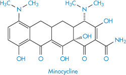
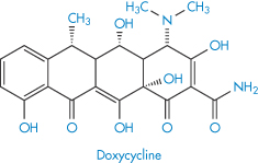
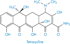
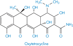
apH 7.4.
bpH 7.5.
The pH dependence of partition coefficients of tetracyclines is more complex than for most drugs, as the tetracyclines are amphoteric.
For slightly simpler amphoteric compounds, such as p-aminobenzoic acid and sulfonamides, the apparent partition coefficient is maximal at the isoelectric point. Figure 4.10 illustrates the variation with pH of log Papp for p-aminobenzoic acid and for two sulfonamides.
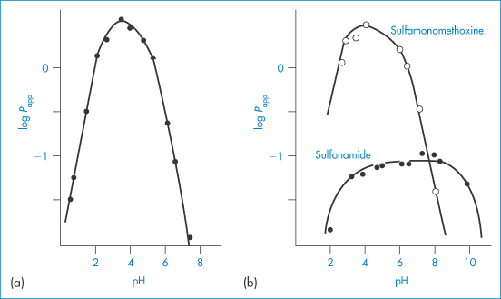
Figure 4.10 (a) Variation of log Papp with pH for p-aminobenzoic acid. (b) Variation of log Papp with pH for sulfamonomethoxine and sulfonamide.
Reproduced with permission from Terada H. Chem Pharm Bull 1972;20:765.
The participation of the zwitterionic species in the partitioning can be excluded because of its low concentration, thus Kt → 0 in Scheme 4.1. From this we obtain P and Papp as follows:
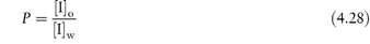
and
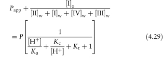
If Kt → 0,
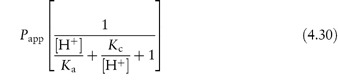
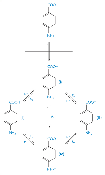
Scheme 4.1 Partitioning of p-aminobenzoic acid. Ka, Kb, Kc and Kd are microdissociation constants for each equilibrium and the relation between them is  where K1 and K2 are composite or macroscopic acid dissociation constants and Kt is the tautomeric constant between the zwitterionic and neutral forms.
Reproduced with permission from Terada H. Partition behavior of p-aminobenzoic acid and sulfonamides at various pH values. Chem Pharm Bull 1972;20:765.
Passive diffusion of sulfonamides into human red cells is determined by plasma drug binding and lipid solubility. Apparent partition coefficients between chloroform and water at pH 7.4 show an almost linear relation with penetration constant for sulfonamides and a number of other acids. Penetration rates of sulfonamides into the aqueous humour and cerebrospinal fluid also correlate with partition coefficients (Fig. 4.11); moreover, the antibacterial effects of a range of fatty acids and esters towards B. subtilis correlate with octanol/water partition coefficients.
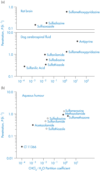
Figure 4.11 (a) Penetration rates of sulfonamides from plasma into rat brain and into canine cerebrospinal fluid. (b) Penetration rates of sulfonamides from plasma into aqueous humour for the rabbit (Ο) and for the rat (●) against partition coefficients (chloroform/water).
(a) Dog cerebrospinal fluid data from Rall DP. J Pharm Exp Ther 1959;125:185.
(b) Data from Wistrand PJ. Acta Pharmacol Toxicol 1960;17:337 and Sorsby A. Br J Ophthalmol 1949;33:347.
There are many quantitative relationships between physiological action and log P or log Papp. A few examples are given in Box 4.1.
Local anaesthetic action on peripheral nerves is also proportional to P since the un-ionised form must diffuse across the continuous cell layer of the perineurium. Once across the perineurium, the molecules ionise and they combine with the receptors in the nerve membrane in their ionised form.
Box 4.1 Relationships between physiological action and partition coefficient |
Absorption of acidic drugs from the colon may be quantified according to P and pKa by the equation
Absorption of bases from the small intestine has been similarly treated:
|
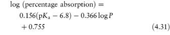
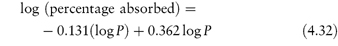
The toxicity of some agents such as X-ray contrast media and penicillins has also been related to lipophilicity. Rates of entry into the brain of X-ray contrast agents used in cerebral angiography are proportional to P, and P correlates with clinical neurotoxicity. Figure 4.12 shows the positive relationship between toxicity of the penicillins and partition coefficient.
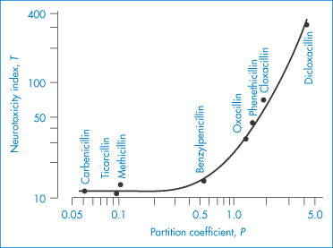
Figure 4.12 Relation of neurotoxicity to the hydrophobic character of various penicillins: the hydrophobic character is measured by the partition coefficient P and toxicity by a neurotoxicity index, T.
Reproduced from Weihrauch TR et al. Cerebral toxicity of penicillins in relation to their hydrophobic character. Arch Pharmacol (NS) 1975;289:55, with kind permission from Springer Science and Business Media.
4.10.2 Sorption
Figure 4.13 summarises the physicochemical problems in the use of preservative molecules in formulations. Solubility and partition coefficients of ionised species are determined, as we have seen, by the pH and ionic strength of the system. In this example, partitioning may occur from the aqueous phase to the oily phase of an emulsion, to the micellar phase of a surfactant, or to a closure. Adsorption may also occur on to container closures and suspended solid particles.
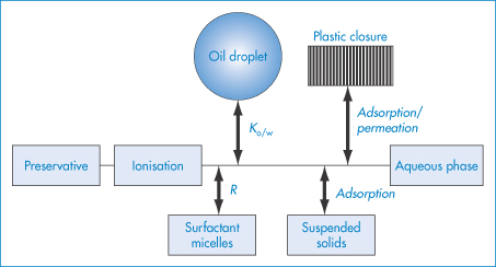
Figure 4.13 The potential fate of preservative molecules in pharmaceutical products. Much depends on the state of ionisation of the molecules. Partitioning into oil droplets or surfactant micelles can occur, as well as adsorption on to suspended solids. Adsorption, sorption or permeation of plastic closures can occur, leaving the less active form in the aqueous phase.
Permeation of antimicrobial agents into rubber stoppers and other closures is another example of partitioning. Although rubber is an amorphous solid, partitioning between the aqueous phase and rubber depends, as in liquid systems, on the relative affinities of the solute for each phase.
Glyceryl trinitrate, a volatile drug with a chloroform/water partition coefficient of 109, diffuses from simple tablet bases into the walls of plastic bottles and into plastic liners used in packaging tablets. This partitioning can be prevented if there is included in the tablet formulation an agent (such as polyoxyethylene glycol) that complexes with the drug substance, thereby increasing its affinity for the ‘tablet phase’ – in other words, reducing its escaping tendency or ‘fugacity’. Significant losses of glyceryl trinitrate have been detected when the drug was given as an infusion through plastic giving sets from a plastic reservoir, the absorption (of as much as 50% of the drug) resulting in the necessity to use unusually high doses of the drug.
Some relation has been found between the rate of sorption by poly(vinyl chloride) (PVC) bags of a series of drugs and their hexane/water partition coefficients.23 Table 4.20 shows the data for sorption of 100 cm3 PVC infusion bags (equivalent to 11 g of PVC). In the table, Papp values have been calculated from
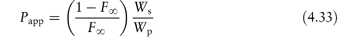
where Ws is the weight of solution in contact with a given weight Wp of plastic and F∞ is the equilibrium fraction of drug remaining in solution. Only the un-ionised form of the drug is sorbed; the kinetics of the process can be accounted for by considering the diffusion of the molecules in the plastic matrix.
Table 4.20 Sorption into poly(vinyl chloride) and partitioning of drugs
Compound | Initial rate of sorption (10−2 h−1) | Extent of sorption at equilibrium (%) | log Papp | log P (hexane/water) |
Medazepam | 51 | 85 | 1.7 | 2.9 |
Diazepam | 27 | 90 | 1.9 | 0.9 |
Warfarin (pH 2–4) | 22 | 90 | 1.9 | 0.2 |
Glyceryl trinitrate | 20 | 83 | 1.6 | 0.2 |
Thiopental (pH 4) | 6 | 73 | 1.4 | 0.1 |
Oxazepam | 4.6 | 46 | 0.9 | −0.1 |
Nitrazepam | 4.1 | 47 | 0.9 | −0.1 |
Hydrocortisone acetate | 0 | 0 | – | −1.2 |
Pentobarbital (pH 4) | 0 | 0 | – | −1.3 |
Reproduced with permission from Illum L, Bundgaard H. Sorption of drugs by plastic infusion bags. Int J Pharm 1982;10:339–351. Copyright Elsevier 1982.
There are concerns over phthalates in medical devices, including diethylhexylphthalate (DEHP), used in medical products made of PVC such as IV bags, blood bags and tubing. DEHP can ‘leach’ out of PVC into liquids such as IV fluids, especially in the presence of formulations containing additives such as surfactants, as with Cremophor EL in Taxol. Figure 4.14 illustrates some of the problems that can occur in giving sets.
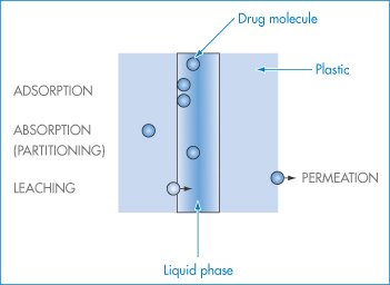
Figure 4.14 Diagram showing opportunities in plastic systems for adsorption of drug molecules, partitioning into (absorption) and eventually permeation through the plastic. Leaching of molecules from the plastic also may occur.
4.10.3 A chromatographic model for the biophase
Octanol/water partition coefficients, as we have seen, have been useful predictors of biological activity. In spite of this it has been suggested that bulk liquid phases may not be the most appropriate models for a structured biophase such as a biological membrane, and chromatographic stationary phases have been proposed as an alternative because of the structuring of the ‘membranous’ hydrophobic chains.
4.10.4 Calculating log P from molecular structures
The large number of methods used to calculate log P values have been elegantly reviewed by Leo et al.21 The method proposed in 1964 by Fujita et al.24 used values for the ‘parent’ molecule and values for substituents gathered by analysis of thousands of values of log P for homologous and other series. In this method of ‘substituents’, log P is considered to be an additive-constitutive free-energy-related property, where one can define Π for substituent X as the difference between the log P values for the parent solute and the compound with the substituent:

By definition Π(H) = 0. For example,
compared with a measured value of 2.45.
The fragmental method developed by Rekker and Mannhold25 uses the contributions of simple fragments. This may be illustrated by the example:

where PE1 is a ‘proximity effect’, an adjusting fraction for polar fragments in non-polar surroundings. So
compared with a measured value of 1.34.
A method based on the surface areas of molecules has also been proposed to obtain measures of log P in a manner analogous to the calculation of solubility.26 Computer programs for calculation of log P are also in use and are described in detail in Leo et al.’s (1993) review.21
4.10.5 Drug distribution into human milk
The distribution of drugs into the milk of breastfeeding mothers is of obvious importance. Nearly all drugs find their way into milk and it is, therefore, useful to be able to predict which of them will achieve high concentrations in milk in relation to their plasma level, defined in one model27 described below as the milk:plasma (M/P) ratio (Table 4.21). Three key parameters are the pKa of the drug, plasma protein binding and the octanol/water partition coefficients of the drugs. Protein binding is the most important single predictor, an increase in M/P ratios generally being found as protein binding decreases. The equations used to calculate M/P ratios are shown in Box 4.2.
Table 4.21 Distribution of drugs into milk: the M/P ratiob
Drug | M/P |
Acidic drugs | |
Carbenicillin | 0.02 |
Ethosuximide | 0.78 |
Ibuprofen | 0 |
Paracetamol | 0.76 |
Valproic acid | 0.05 |
Basic drugs | |
Amitriptyline | 0.83 |
Atenolol | 0.32 |
Cimetidine | 1.7 |
Clonazepam | 0.33 |
Codeine | 2.16 |
Lamotrigine | 0.4–0.45 |
Morphine | 2.46 |
Verapamil | 0.6 |
Vigabatrin | 0.01–0.05 |
Neutral drugs | |
Alcohol | 0.89 |
Digoxin | 0.55 |
Medroxyprogesterone | 0.72 |
Norethisterone | 0.19 |
Prednisolone | 0.13 |
b M/P = Milk : plasma drug concentration ratio.
Reproduced from Atkinson HC, Begg EJ. Prediction of drug distribution into human milk from physicochemical characteristics. Clin Pharmacokinet 1990;18:151–167, with kind permission from Springer Science and Business Media.
Box 4.2 The calculation of milk:plasma ratios |
The two key equations, each with three independent variables, are as follows: For basic drugs:
For acidic drugs:
where Mu/Pu = milk:plasma unbound drug fu,p = fraction of drug unbound in plasma fu,m = fraction of drug unbound in milk K = (0.955/fu,m) + [0.045Papp(milk/lipid)] Papp = apparent partition coefficient at pH 7.2 Few measurements of fu,m and Papp(milk/lipid) have been made, but these parameters can be predicted from fu,p and log P.28 It is clear from equations (4.35) and (4.36) that there is a degree of empiricism about these equations, which arises in their derivation from the fitting of data sets based on the independent variables. The ratio Mu/Pu can be obtained from the modified Henderson–Hasselbalch equation. For basic drugs,
and for acidic drugs,
where pHm and pHp are the pH values of milk and plasma, respectively. Milk has a mean pH of 7.2, slightly lower than that of plasma at 7.4. For neutral drugs the predicted Mu/Pu ratio would be unity, since the distribution of unbound un-ionised drugs would not be expected to be altered by pH gradients. |
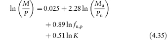
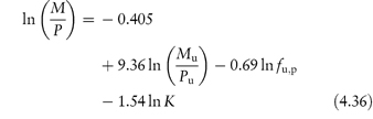
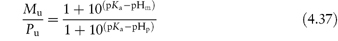
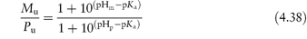
|
|

Summary
Definitions of solubility, modes of expression of solubility and means of estimating solubility from the surface area of molecules were some of the key subjects discussed in this chapter. Molecular shape factors and substituents on molecules affect solubility, one of the key parameters of a drug substance. Effects such as solvation (or hydration in aqueous media) and the effects of additives on solubility are also dealt with, but perhaps the most important effect of all is that of pH on the solubility of ionisable drugs. This is treated in detail, and equations for acids, bases and zwitterions are considered. An understanding of pH–solubility relationships is vital to predicting the behaviour of ionic drugs in pharmaceutical formulations and in the body.
When additives, such as surfactants and CDs, do not achieve appropriate levels of practical solubility, we can resort to the use of cosolvents. The relative advantages and disadvantages of these different approaches to formulating a solution have to be considered, but in the last analysis other factors such as stability may determine which is the best approach to achieve a satisfactory solution formulation.
We have discussed the partitioning of a drug between immiscible phases and the importance of the partition coefficient (and its logarithm, log P) in defining the relative affinities of a solute for an aqueous and a non-aqueous or lipid phase, and as an important measure of the lipophilicity of a drug. Correlations between the partition coefficients and physiological action of several classes of drug have been examined. We have also seen the role of log P in quantifying a wide variety of diverse processes such as the extent to which a drug will adsorb on to container closures or distribute into human milk. Further examples of the importance of partitioning between aqueous and oily phases in, for example, emulsions and micellar systems will be examined in later chapters.
References
1. Amidon GL et al. Solubility of nonelectrolytes in polar solvents. II. Solubility of aliphatic alcohols in water. J Pharm Sci 1974;63:1858–1866.
2. Amidon GL. Theoretical calculation of heats of complexation in carbon tetrachloride. J Pharm Sci 1974;63:1520–1523.
3. Amidon GL et al. Solubility of nonelectrolytes in polar solvents. V. Estimation of the solubility of aliphatic monofunctional compounds in water using a molecular surface area approach. J Phys Chem 1975;79:2239–2246.
4. Hermann RB. Theory of hydrophobic bonding. II. Correlation of hydrocarbon solubility in water with solvent cavity surface area. J Phys Chem 1972;76:2754–2759.
5. Hermann RB. Theory of hydrophobic bonding. I. Solubility of hydrocarbons in water, within the context of the significant structure theory of liquids. J Phys Chem 1971;75:363–368.
6. Franks F. In: Duckworth RD (ed.) Water Relations of Foods. London: Academic Press; 1975.
7. Bergstrom CAS et al. Accuracy of calculated pH-dependent aqueous drug solubilities. Eur J Pharm Sci 2004;22:387–398.
8. Tse RL, Lee MW. pH of infusion fluids: a predisposing factor in thrombophlebitis. J Am Med Assoc, 1971; 215: 642.
9. Green AL. Ionisation constants and water solubilities of some aminoalkyl phenothiazine tranquillizers and related compounds. J Pharm Pharmacol 1967;19:10–16.
10. Bennett LJ, Miller KW. Application of regular solution theory to biomembranes. J Med Chem 1974;17:1124–1125.
11. Scott RS. Solutions of nonelectrolytes. Annu Rev Phys Chem 1956;7:43–66.
12 Krause GM, Cross JM, J Am Pharm Assoc, 1951; 40; 137.
13. Miyako Y et al. Solubility enhancement of hydrophobic compounds by cosolvents: role of solute hydrophobicity on the solubilisation effect. Int J Pharm 2010;393:48–54.
14. Mizuuchi H et al. Room temperature ionic liquids and their mixtures: potential pharmaceutical solvents. Eur J Pharm Sci 2008;33:326–331.
15. Loftsson T, Brewster ME. Pharmaceutical applications of cyclodextrins. 1. Drug solubilization and stabilization. J Pharm Sci 1996;85:1017–1025.
16. Kurkov SV, Loftsson T. Cyclodextrins. Int J Pharm 2013;453:167–180.
17. Yang W, de Villiers MM. The solubilization of the poorly water soluble drug nifedipine by water soluble 4-sulphonic calix[n]arenes. Eur J Pharm Biopharm 2004;586:29–36.
18. Serajuddin ATM. Salt formation to improve drug solubility. Adv Drug Del Rev 2007;59:603–616.
19. Boyd E. Predictive Toxicometrics. Bristol: Scientechnica; 1972.
20. Leo AJ et al. Partition coefficients and their uses. Chem Rev 1971;71:525–616.
21. Leo AJ et al. Calculating log Poct from structures. Chem Rev 1993; 931:281–306.
22. Ferguson J. The use of chemical potentials as indices of toxicity. Proc R Soc Lond (Biol) 1939; 127:387–404.
23. Illum L, Bundgaard H. Sorption of drugs by plastic infusion bags. Int J Pharm 1982;10:339–351.
24. Fujita T et al. A new substituent constant, π, derived from partition coefficients. J Am Chem Soc 1964;86:5175–5180.
25. Rekker R, Mannhold R. Calculations of Drug Lipophilicity. Weinheim: VCH; 1992.
26. Broto P et al. Molecular structures: perception, autocorrelation descriptor and SAR studies. Perception of molecules: topological structure and 3-dimensional structure. Eur J Med Chem 1984;19:61–65.
27. Atkinson HC, Begg EJ. Prediction of drug distribution into human milk from physicochemical characteristics. Clin Pharmacokinet 1990;18:151–167.
28. Begg EJ et al. Prospective evaluation of a model for the prediction of milk: plasma drug concentrations from physicochemical characteristics. Br J Clin Pharmacol 1992; 33:501–505.
Stay updated, free articles. Join our Telegram channel

Full access? Get Clinical Tree


