Quentin J. Baca and David E. Golan

Pharmacodynamics is the term used to describe the effects of a drug on the body. These effects are typically described in quantitative terms. The previous chapter considered the molecular interactions by which pharmacologic agents exert their effects. The integration of these molecular actions into an effect on the organism as a whole is the subject addressed in this chapter. It is important to describe the effects of a drug quantitatively in order to determine appropriate dose ranges for patients, as well as to compare the potency, efficacy, and safety of one drug to that of another.
 Admiral X is a 66-year-old retired submarine captain with a 70 pack–year smoking history (two packs a day for 35 years) and a family history of coronary artery disease. He takes daily atorvastatin to reduce his cholesterol level and aspirin to reduce his risk of coronary artery occlusion.
One day, while working in his wood shop, Admiral X begins to feel tightness in his chest. The feeling rapidly becomes painful, and the pain radiates down his left arm. He calls 911, and an ambulance transports him to the local emergency department. After evaluation, it is determined that Admiral X is having an anterior myocardial infarction. Because Admiral X cannot be transferred to a hospital with a cardiac catheterization laboratory within 120 minutes of first medical contact, and he has no relative contraindications to thrombolytic therapy (such as uncontrolled hypertension, history of stroke, or recent surgery), the physician initiates therapy with both a thrombolytic agent, tissue-type plasminogen activator (tPA), and an anticoagulant, heparin. Because of their low therapeutic indices, improper dosing of both of these drugs can have dire consequences (hemorrhage and death). Therefore, Admiral X is closely monitored, and the pharmacologic effect of the heparin is measured periodically by testing the partial thromboplastin time (PTT). Admiral X’s symptoms resolve over the next several hours, although he remains in the hospital for monitoring. He is discharged after 4 days in the hospital; his discharge medications include atorvastatin, aspirin, atenolol, lisinopril, and clopidogrel for secondary prevention of myocardial infarction.
Questions
1. How does the molecular interaction of a drug with its receptor determine the potency and efficacy of the drug?
2. Why does the fact that a drug has a low therapeutic index mean that the physician must use greater care in its administration?
3. What properties of certain drugs, such as aspirin, allow them to be taken without monitoring of plasma drug levels, whereas other drugs, such as heparin, require such monitoring?

The study of pharmacodynamics is based on the concept of drug–receptor binding. When either a drug or an endogenous ligand (such as a hormone or neurotransmitter) binds to its receptor, a response may result from that binding interaction. When a sufficient number of receptors are bound (or “occupied”) on or in a cell, the cumulative effect of receptor “occupancy” may become apparent in that cell. At some point, all of the receptors may be occupied, and a maximal response may be observed (an exception is the case of spare receptors; see below). When the response occurs in many cells, the effect can be seen at the level of the organ or even the patient. But this all starts with the binding of drug or ligand to a receptor (for the purpose of discussion, “drug” and “ligand” will be used interchangeably for the remainder of this chapter). A model that accurately describes the binding of drug to receptor would therefore be useful in predicting the effect of the drug at the molecular, cellular, tissue (organ), and organism (patient) levels. This section describes one such model.
Consider the simplest case, in which the receptor is either free (unoccupied) or reversibly bound to drug (occupied). We can describe this case as follows:

where L is ligand (drug), R is free receptor, and LR is bound drug–receptor complex. At equilibrium, the fraction of receptors in each state is dependent on the dissociation constant, Kd, where Kd = koff/kon. Kd is an intrinsic property of any given drug–receptor pair. Although Kd varies with temperature, the temperature of the human body is relatively constant, and it can therefore be assumed that Kd is a constant for each drug–receptor combination.
According to the law of mass action, the relationship between free and bound receptor can be described as follows:
where [L] is free ligand concentration, [R] is free receptor concentration, and [LR] is ligand–receptor complex concentration. Because Kd is a constant, some important properties of the drug–receptor interaction can be deduced from this equation. First, as ligand concentration is increased, the concentration of bound receptors increases. Second, and not so obvious, is that as free receptor concentration is increased (as may happen, for example, in disease states or upon repeated exposure to a drug), bound receptor concentration also increases. Therefore, an increase in the effect of a drug can result from an increase in the concentration of either the ligand or the receptor.
The remainder of the discussion in this chapter, however, assumes that the total concentration of receptors is a constant, so that [LR] + [R] = [Ro]. This allows Equation 2-2 to be arranged as follows:
Solving for [R] and substituting Equation 2-3 into Equation 2-2 yields:
Note that the left side of this equation, [LR]/[Ro], represents the fraction of all available receptors that are bound to ligand.
Figure 2-1 shows two plots of Equation 2-4 for the binding of two hypothetical drugs to the same receptor. These plots are known as drug–receptor binding curves. Figure 2-1A shows a linear plot, and Figure 2-1B shows the same plot on a semilogarithmic scale. Because drug responses occur over a wide range of doses (concentrations), the semilog plot is often used to display drug–receptor binding data. The two drug–receptor interactions are characterized by different values of Kd. In this case, KdA < KdB.
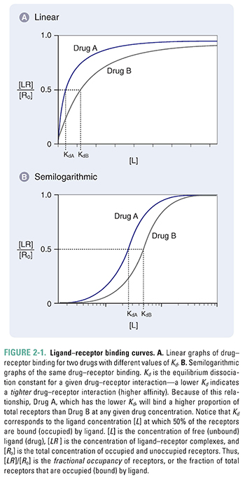
Notice from Figure 2-1 that maximal drug–receptor binding occurs when [LR] is equal to [Ro], or [LR]/[Ro] = 1. Also notice that, according to Equation 2-4, when [L] = Kd, then [LR]/[Ro] = Kd/2Kd = ½. Thus, Kd can be defined as the concentration of ligand at which 50% of the available receptors are occupied.

The pharmacodynamics of a drug can be quantified by the relationship between the dose (concentration) of the drug and the organism’s (patient’s) response to that drug. One might intuitively expect the dose–response relationship to be related closely to the drug–receptor binding relationship, and this turns out to be the case for many drug–receptor combinations. Thus, a useful assumption at this stage of discussion is that the response to a drug is proportional to the concentration of receptors that are bound (occupied) by the drug. This assumption can be quantified by the following relationship:

where [D] is the concentration of free drug, [DR] is the concentration of drug–receptor complexes, [Ro] is the concentration of total receptors, and Kd is the equilibrium dissociation constant for the drug–receptor interaction. (Note that the right side of Equation 2-5 is equivalent to Equation 2-4, with [D] substituted for [L].) The generalizability of this assumption is examined below.
There are two major types of dose–response relationships—graded and quantal. The difference between the two types is that graded dose–response relationships describe the effect of various doses of a drug on an individual, whereas quantal relationships show the effect of various doses of a drug on a population of individuals.
Graded Dose–Response Relationships
Figure 2-2 shows graded dose–response curves for two hypothetical drugs that elicit the same biological response. The curves are presented on both linear and semilogarithmic scales. The curves are similar in shape to those in Figure 2-1, consistent with the assumption that response is proportional to receptor occupancy.
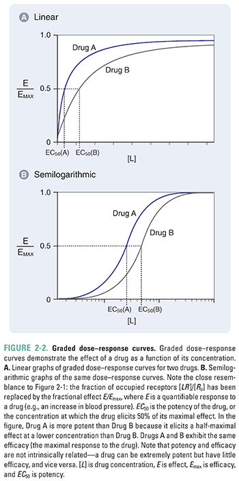
Two important parameters—potency and efficacy—can be deduced from the graded dose–response curve. The potency (EC50) of a drug is the concentration at which the drug elicits 50% of its maximal response. The efficacy (Emax) is the maximal response produced by the drug. In accordance with the assumption stated above, efficacy can be thought of as the state at which receptor-mediated signaling is maximal and, therefore, additional drug will produce no additional response. This usually occurs when all the receptors are occupied by the drug. Some drugs, however, are capable of eliciting a maximal response when less than 100% of the drug’s receptors are occupied; the remaining receptors can be called spare receptors. This concept is discussed further in the text that follows. Note again that the graded dose–response curve of Figure 2-2 bears a close resemblance to the drug–receptor binding curve of Figure 2-1, with EC50 replacing Kd and Emax replacing Ro.
Quantal Dose–Response Relationships
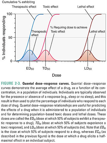
The quantal dose–response relationship plots the fraction of the population that responds to a given dose of drug as a function of the drug dose. Quantal dose–response relationships describe the concentrations of a drug that produce a given effect in a population. Figure 2-3 shows an example of quantal dose–response curves. Because of differences in biological response among individuals, the effects of a drug are seen over a range of doses. The responses are defined as either present or not present (i.e., quantal, not graded). Endpoints such as “sleep/no sleep” or “alive at 12 months/not alive at 12 months” are examples of quantal responses; in contrast, graded dose–response relationships are generated using scalar responses such as change in blood pressure or heart rate. The goal is to generalize a result to a population rather than to examine the graded effect of different drug doses on a single individual. Types of responses that can be examined using the quantal dose–response relationship include effectiveness (therapeutic effect), toxicity (adverse effect), and lethality (lethal effect). The doses that produce these responses in 50% of a population are known as the median effective dose (ED50), median toxic dose (TD50), and median lethal dose (LD50), respectively.
Stay updated, free articles. Join our Telegram channel

Full access? Get Clinical Tree


