Epidemiology
Neal Nathanson
William J. Moss
Basic Definitions and Methods
Epidemiology deals with the occurrence of diseases in populations. Historically, epidemics of viral disease were recognized long before their causal agents were discovered, and viral epidemiology was one of the first aspects of the science of virology to be developed. Evolving insights into the pathogenesis and molecular aspects of virology have provided an increasingly rational basis for understanding the epidemiology of viruses. In this chapter, the biology of viral infections is used to explain the essentials of viral epidemiology.
Incidence and Prevalence
The quantification of disease occurrence is the cardinal feature of epidemiology. To accomplish this, the concept of rates was introduced, and rates have become the basic coinage of epidemiology (Fig. 12.1). Rates are fractions in which the numerator is the number of cases of disease and the denominator is a measure of the population. The incidence rate (also called the attack rate for acute infectious diseases) is used to quantify the number of new infections. A population and a time frame are defined, and the number of new cases in that population during that interval of time is counted. Note that the denominator includes both the size of population and time frame, and is often expressed as person-years (or any other standard interval of time; e.g., “thousand person-years” or “hundred person-weeks”). The incidence rate is then expressed as “cases per thousand person-years” or a similar term. Also note that the time element may be omitted in expressing incidence; the reader must then determine by context the time frame used.
Prevalence, technically not a rate but a ratio, refers to the total number of cases present within a specified time interval. Thus, the numerator in prevalence includes not just new cases but cases carried forward from the period prior to the specified time interval. When point prevalence is computed, a particular narrow time frame is selected, and the population recorded for that time frame constitutes the denominator. All cases “prevalent” on that date constitute the numerator. Prevalence is expressed as a ratio such as “cases per million”; note that there is no time parameter in this ratio.
Changes in incidence and prevalence may be divergent. A control program for human immunodeficiency virus (HIV) infection, for example, could decrease HIV incidence within a population through effective preventative measures but increase the prevalence of HIV infection through access to antiretroviral therapy and improved survival.
In epidemiology, consistency is a virtue. When cases and populations are counted prior to computing rates, care must be
taken to use the same definition for numerator and denominator. Persons counted in the denominator should be at risk to be a case in the numerator if infected. For instance, if incidence is computed for the population of Philadelphia for 2011, a case hospitalized in the city but resident outside the city would not be counted. A case with onset in December 2010 but still ill in 2011 would not be counted as an incident case but would be a prevalent case.
taken to use the same definition for numerator and denominator. Persons counted in the denominator should be at risk to be a case in the numerator if infected. For instance, if incidence is computed for the population of Philadelphia for 2011, a case hospitalized in the city but resident outside the city would not be counted. A case with onset in December 2010 but still ill in 2011 would not be counted as an incident case but would be a prevalent case.
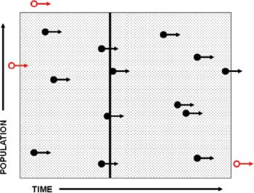 Figure 12.1. Computation of incidence rate and prevalence ratio. The shaded area defines a population and a time frame that can be expressed as person-time units. Cases of disease are indicated by circles (placed according to the date of their onset) and arrows for duration of illness. Solid circles would be counted for computation of incidence, whereas open circles would be excluded because they had onset outside the designated time frame or were resident outside the population boundaries. Incidence equals the number of cases divided by population-time units. Prevalence would be determined by a single vertical line across the hatched area: Cases active at that time point would be divided by the size of the population to compute the prevalence. |
What distinguishes infectious disease epidemiology from chronic disease epidemiology is that the former accounts for dependent happenings, a term introduced by Ronald Ross,102 in which the incidence of a disease depends on its prevalence within a population.45 Traditional epidemiologic and statistical methods that infer relationships between exposure and disease outcome assume that the outcome in one individual is independent of the outcome in other individuals, an assumption that is invalid for communicable viral infections.54,82
Sources of Data
In practice, the accurate collection of data for the computation of rates is often a major undertaking, whereas the computations are relatively simple. Furthermore, the practicing epidemiologist must frequently work with incomplete and inaccurate information. In most developed countries, denominator (population) information is usually good, and numerator (case) information is the major problem. In resource-limited settings, accurate population data may be unavailable.
For infectious (viral) diseases, there are several sources of case data. Passive surveillance denotes the continuous reporting of disease by healthcare workers. By law, many viral diseases are designated as “reportable,” and in theory, the reporting of all cases is required. Cases are reported by practicing physicians, hospitals, or laboratories to local health jurisdictions, which in turn relay reports to a central state office whence they are transmitted to a national center (e.g., the U.S. Centers for Disease Control and Prevention). The weakest link is the initial report; in practice, only a small fraction of cases of many common viral diseases (such as 10%–15% of measles or hepatitis B cases) are reported to the national center (called the reporting efficiency). However, if the proportion of cases reported is consistent between geographic locales and between years, these reports may be used to monitor trends. Consistency is an important caveat, because the proportion of cases reported may increase if the absolute number of cases decreases. Changes in the case definition also may result in spurious changes in surveillance data. Reporting of certain rare or serious diseases, such as poliomyelitis or acquired immunodeficiency syndrome (AIDS), is often close to 100%; in such instances, reported cases can be used with much greater confidence for calculation of rates. Within increasing interest in the pandemic spread of respiratory viruses and the emergence of new zoonotic viral pathogens, global disease surveillance networks have been established to provide data on disease incidence and transmission in real time,14 including the Program for Monitoring Emerging Diseases (ProMED) and the World Health Organization’s Global Outbreak Alert and Response Network (GOARN).
Active case detection through epidemic investigation is the traditional approach to collecting information on outbreaks of disease. Such investigations are usually initiated by public health authorities but may be instigated by healthcare workers or patient families. The investigation is tailored to the situation and to the resources at hand, although experience has set certain guidelines, particularly for recurring outbreaks such as food-borne diseases. The purpose of such studies is several: (a) to classify the illness and determine the causative organism, (b) to assess the extent of the outbreak and its economic and health impact, (c) to abort the outbreak or prevent recurrent episodes, and (d) to inform or reassure the public. The first recognition of a new disease or isolation of a previously unknown virus has been accomplished as a result of an epidemic investigation. Examples are the identification of Lassa virus; Marburg virus; Sin Nombre virus (SNV), a hantavirus that is the cause of acute pulmonary syndrome; severe acute respiratory syndrome (SARS)-coronavirus; and the 2009 H1N1 influenza virus.
Serological surveys may be used to detect the footprints that a virus leaves in a population. Serosurveys are particularly useful for viruses because most viral infections leave an imprint on all infected individuals—that is, the presence of immunoglobulin G (IgG) antibody, which often is life long. Because many viruses cause asymptomatic infections or nondescript illnesses in addition to diagnosable diseases, serological surveys identify inapparent as well as apparent infections. Incident viral infection can be identified using assays for immunoglobulin M (IgM) antibody or antibody avidity, whereas IgG antibodies indicate prior infection or vaccination.
Cohort and Case-Control Study Designs
Modern epidemiology has made one outstanding contribution to the discipline—namely, the extension of hypothesis testing from the laboratory to populations. In general, the epidemiologist
attempts to test the hypothesis that one or more population variables influence the occurrence of a specified disease and, if so, to quantify this effect and estimate confidence limits. There are two general designs used for such studies: cohort and case-control studies. The essence of these designs is summarized next, and the reader is referred to appropriate texts for methodological exposition.35
attempts to test the hypothesis that one or more population variables influence the occurrence of a specified disease and, if so, to quantify this effect and estimate confidence limits. There are two general designs used for such studies: cohort and case-control studies. The essence of these designs is summarized next, and the reader is referred to appropriate texts for methodological exposition.35
Table 12.1 Hypothetical Data to Illustrate Computations for a Cohort and a Case-Control Study of Vaccine Efficacy | |||||||||||||||||||||||||||||||||||||||||||||||||||||||
|---|---|---|---|---|---|---|---|---|---|---|---|---|---|---|---|---|---|---|---|---|---|---|---|---|---|---|---|---|---|---|---|---|---|---|---|---|---|---|---|---|---|---|---|---|---|---|---|---|---|---|---|---|---|---|---|
| |||||||||||||||||||||||||||||||||||||||||||||||||||||||
Cohort Studies
In a cohort study, which may be conducted prospectively or retrospectively, the population is divided into two groups, one with and one without a specified exposure or attribute. Both groups are followed prospectively for the incidence of the disease under study, and incidence rates for both groups are then computed. A hypothetical example is shown in Table 12.1. In this example, the population attribute is immunization against a specified viral disease, and the attack rate in the immunized population is one-third the rate in the unimmunized control group. The relative risk (RR) associated with immunization is 0.33, and vaccine efficacy is 67% [(1 – RR) × 100]. There is one important assumption underlying the validity of such a study: The immunized and unimmunized groups are at equal risk of disease. For various reasons, this assumption may not be correct. Differences in the risk of disease between two study groups may be minimized by random allocation of the exposure (in this case, the vaccine) when that is deemed ethical. However, random allocation of exposure is not possible unless the study is of an intervention. Stratifying each study arm according to parameters such as age, race, and socioeconomic status and then comparing rates for each subgroup can be used to identify inequalities between the two groups. Table 12.2 summarizes one such study of polio vaccine and documents the problems of comparing groups (in this instance, vaccinated and unvaccinated) that are not at equivalent risk of disease (in this instance, poliomyelitis).
More complex study designs are used to measure indirect effects of vaccines or other interventions that affect the transmission of viral pathogens. Such indirect effects include protection of non-vaccinated individuals through decreased transmission from vaccinated individuals, referred to as herd immunity.27 Cluster randomized trials—for example, cohort studies in which communities rather than individuals are randomized to receive the intervention—allow direct measurement of the indirect effects of vaccines by comparing the risk of disease outcomes in nonvaccinated individuals residing in intervention and control communities.44,46
Case-Control Studies
Cohort studies usually require extensive resources and time because they necessitate the enrollment of large numbers of subjects who must be followed for a period of months or years; the less frequent the expectation of disease, the larger the population or longer the follow-up needed. Needless to say, the costs of prospective cohort studies can be great, limiting them to situations such as the introduction of a new drug or vaccine, as illustrated in Table 12.2. Case-control studies can be more cost-effective because they involve smaller numbers of subjects and do not require longitudinal follow-up, particularly if the disease outcome is rare. Table 12.1 shows a simplified version of such a study. In this instance, 100 cases of the study disease and 100 unaffected control subjects are identified and classified according to the exposure or attribute (vaccination) under study. For both vaccinated and unvaccinated individuals, an odds ratio is computed. Because, under certain assumptions, the odds ratios have the same relationship as the rates computed in the prospective study shown in the upper half of Table 12.1,
the relative risk can be estimated as the ratio of the two odds (0.4/1.2 = 0.33). Two assumptions underlie the validity of the case-control design and analysis, specifically the use of the odds ratio as an estimate of relative risk: The two samples (cases and controls) must be representative of the population from which they are drawn, and the incidence of disease must be low so that cases comprise less than 10% of the total population. Because case-control studies are particularly useful to study risk factors for rare diseases, the second assumption is usually correct. The main challenge in designing case-control studies is the choice of a valid and representative control group, a subject considered in depth in epidemiologic texts.35
the relative risk can be estimated as the ratio of the two odds (0.4/1.2 = 0.33). Two assumptions underlie the validity of the case-control design and analysis, specifically the use of the odds ratio as an estimate of relative risk: The two samples (cases and controls) must be representative of the population from which they are drawn, and the incidence of disease must be low so that cases comprise less than 10% of the total population. Because case-control studies are particularly useful to study risk factors for rare diseases, the second assumption is usually correct. The main challenge in designing case-control studies is the choice of a valid and representative control group, a subject considered in depth in epidemiologic texts.35
Table 12.2 The 1954 Field Trial of Poliomyelitis Vaccine: Comparison of Attack Rates for Vaccinated and Unvaccinated Childrena | ||||||||||||||||||||||||||||||
|---|---|---|---|---|---|---|---|---|---|---|---|---|---|---|---|---|---|---|---|---|---|---|---|---|---|---|---|---|---|---|
| ||||||||||||||||||||||||||||||
Basic Biological Concepts
Susceptibility and Immunity
Many acute viral infections confer lifelong immunity. Upon re-exposure after initial infection, there is often reinfection but with minimal virus replication and an anamnestic immune response. Such reinfections are usually covert and almost never severe, resulting in minimal or no shedding of infectious virus. For certain viruses, such as poliovirus or rhinovirus, immunity is type specific and confers little protection against exposure to a different serotype. These simple facts have profound implications for viral epidemiology. For epidemiologic purposes, a population may be divided into three groups: susceptible, infected (and infectious), and immune. Persons infected at any time in the past may be considered immune (recovered) and are exempt from disease and unable to act as links in a transmission chain, whereas susceptible individuals can be infected, become infectious, and experience disease. This compartmentalization of the population is the basis for simple SIR (susceptible, infectious, recovered) models of virus transmission4 that can explain the periodicity in incidence as the outcome of the buildup and decline of susceptible individuals.
Susceptibility may not be present immediately after birth. IgG antibodies are actively transported across the placenta, conferring protective immunity to neonates and young infants. For such viral infections, individuals move from a protected state to a susceptible one in the first year of life. Immunity can then be conferred by vaccination or infection.
Persistent viral infections differ from acute infections because the infected individual may be capable of transmitting infection over many years and may develop disease at any time during virus persistence. In the instance of persistent viruses, the population may be divided into uninfected susceptibles and immune-but-infectious persons who carry serological markers of prior infection but who are still capable of acting as links in the chain of infection. Important examples are hepatitis B virus, HIV, and several herpesviruses (herpes simplex virus, varicella-zoster virus, and cytomegalovirus) that establish latent infection capable of reactivation.
Parameters That Determine Incidence
For acute viral infections, the following three parameters determine incidence: the proportion of the population susceptible, the proportion of the population that is infectious, and the rate of contact between susceptible and infectious individuals, with contact defined as an encounter sufficient for transmission. The proportion of infected persons who become ill—the case infection ratio—determines the proportion of infected persons detected through case surveillance.
Proportion Susceptible
When a population is exposed to an infectious individual with a specific virus, the susceptible part of the population will determine the spread of the agent and account for all new cases. The proportion susceptible will reflect the past history of infection with the specific virus in the population and the past history of immunization for vaccine-preventable viral infections.
Proportion Infectious
The proportion of susceptibles who become infected, and subsequently infectious, during a fixed period of time (e.g., year or season) can vary widely, depending on the dynamics of transmission, which is influenced by the density of susceptibles and contact patterns between susceptible and infectious individuals.
Table 12.3 Estimated Case Infection and Case Fatality Ratios for Selected Viral Infections | |||||||||||||||||||||||||||||
|---|---|---|---|---|---|---|---|---|---|---|---|---|---|---|---|---|---|---|---|---|---|---|---|---|---|---|---|---|---|
|
Rate of Contact Between Susceptible and Infectious Individuals
The rate of contact between susceptible and infectious individuals determines the dynamics of viral spread within a population. This rate depends on the mode of transmission (e.g., respiratory, oral–fecal, sexual, or vector-borne), age-specific contact patterns or networks between individuals, and the distribution of susceptible and infectious individuals within a population. Spatial clustering of susceptible individuals can result in outbreaks despite a high proportion of immune individuals within the population.
Case Infection and Fatality Ratios
The proportion of infections resulting in overt disease—the pathogenicity of the organism—is characteristic for each virus and is strikingly different for different agents. One of the most important contributions of modern laboratory methods to viral epidemiology was the identification of inapparent or subclinical infections and the insight that most infections caused by some viruses were asymptomatic. The relative frequency of subclinical infections is expressed as the case infection ratio—that is, the number of clinical cases per 100 infections. The lethality of disease is a different parameter that represents the virulence of the organism and is designated as the case fatality ratio. The case fatality ratio is the number of deaths attributable to an infection per 100 cases. Table 12.3 lists selected common viral infections and shows estimated case infection ratios and case fatality ratios for each. It is noteworthy that there is no regular relationship between the case infection ratio and severity of illness (i.e., between pathogenicity and virulence). For instance, measles has a very high case infection ratio (>95:100) but a low case fatality ratio in developed countries (<1:1000 in the United States). Conversely, poliomyelitis has a low case infection ratio (<1:100) but a higher case fatality ratio (∼5:100). Determining the case infection ratio is an important objective of outbreak investigations of novel pathogens, such as severe acute respiratory syndrome (SARS)-coronavirus and the 2009 pandemic H1N1 influenza virus. Typically, early in an outbreak, only cases that come to clinical attention are counted as incident cases, resulting in an underestimate of the true incidence. Accurate measurement of subclinical infection requires population-based surveys with laboratory confirmation (e.g., serological surveys).
Incubation, Latent, and Infectious Periods
The course of infection in a single individual can be conveniently divided into several periods.29 The interval from acquisition of infection to onset of illness is the incubation period. Note that “onset of illness” must be explicitly defined for each disease and is often measured by the first day on which pathognomonic signs or symptoms are reported. The interval from acquisition of infection to onset of infectiousness is the latent period. For most viral diseases, the latent period is shorter than the incubation period. Consequently, the infected individual begins to shed virus prior to the onset of illness (smallpox is a notable exception) and continues to shed during and sometimes after recovery from the acute illness. The effectiveness of quarantine measures is reduced when the latent period is significantly shorter than the incubation period as the infectious individual goes unrecognized. The period during which the infected person is potentially infectious for others is the infectious period.
Incubation periods for any viral disease vary around the mean, as illustrated in Figure 12.2. When a frequency distribution of individual incubation periods is plotted, it usually has a longer tail at the high end of the distribution (right skewed). If the frequency is plotted against the logarithm of time, the data often approximate a normal distribution.104 This log-normal distribution is characteristic of the incubation periods of many viral infections.60
Generation Time and Serial Interval
The average period between infection of an individual and transmission to others is the generation time or transmission interval. From studies of selected outbreaks, the average interval between onsets of successive waves of cases (called the serial interval) has been determined, and the generation time is often assumed to be equal to this interval as the best approximation available. This is because it is often impossible to know the exact time of infection. These relationships are shown in Figure 12.3 for a typical acute viral infection.
Transmission of Viruses
There are two major patterns of transmission into which viruses may be classified: viruses maintained in a single species and viruses that alternately infect different host species. There
are a few apparent exceptions, such as rabies and influenza viruses, which spread across species boundaries; however, even in these instances, cycles of transmission between different species may be self-contained. For agents that infect humans, a second distinction may be made between those viruses that rely on human transmission for their perpetuation (the majority) and those viruses maintained in an extrahuman cycle for which humans are a dead-end host. Examples of these patterns are set forth in Table 12.4.
are a few apparent exceptions, such as rabies and influenza viruses, which spread across species boundaries; however, even in these instances, cycles of transmission between different species may be self-contained. For agents that infect humans, a second distinction may be made between those viruses that rely on human transmission for their perpetuation (the majority) and those viruses maintained in an extrahuman cycle for which humans are a dead-end host. Examples of these patterns are set forth in Table 12.4.
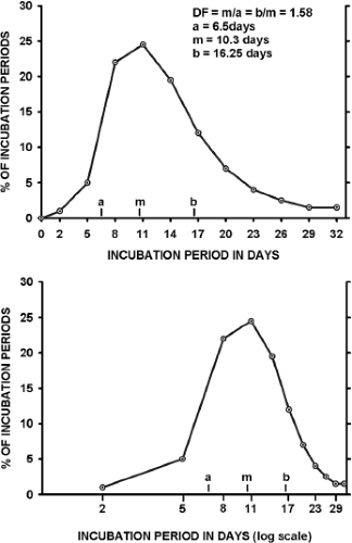 Figure 12.2. Log-normal distribution of incubation periods. Upper panel: Incubation period distribution is shown for poliomyelitis; there is a right-hand tail. Lower panel: The same incubation periods when plotted on a logarithmic scale. Logarithmic incubation period approximates a normal distribution, and the standard deviation may be computed (on the logarithmic scale). The dispersion factor (DF), a measure of the variation of incubation periods, is the antilogarithm of the standard deviation. The mean (m) is shown, together with the standard deviation (points a and b on the graph). The log DF equals the interval (log m to log a) or the interval (log b to log m). In this instance, m is about 10.3 days, a is 6.5 days, b is 16.25 days, and DF is 1.58—that is, about two-thirds of the incubation periods fall into the range (1.58 × mean) to (mean/1.58). (Data from Aycock WL, Luther EH. The incubation period of poliomyelitis. J Prev Med 1929;3:103–120; Casey AE. The incubation period in epidemic poliomyelitis. JAMA 1942;120:805–807; Horstmann DM, Paul JR. The incubation period in human poliomyelitis and its implications. JAMA 1947;135:11–14; Nathanson N, Langmuir AD. The Cutter incident. Am J Hyg 1963;78:16–28; and Sartwell PE. The incubation period of poliomyelitis. Am J Public Health Nations Health 1952;42:1403–1408, with permission.) |
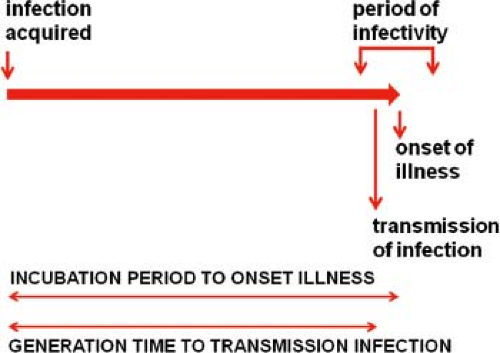 Figure 12.3. Incubation period and generation time. Incubation period is the interval between acquisition of infection and onset of illness, whereas generation time is the interval between acquisition of infection and transmission to another person. This diagram shows the mean for each parameter; in practice, there is a spread around this mean. |
Viruses Maintained Within a Single Host Population
Each virus has characteristic modes of host-to-host transmission: (a) direct person-to-person transmission through respiratory, fecal–oral, sexual, blood, or from mother to child, or (b) indirect transmission through fomites or vectors. Viruses that cause acute short-term infections require efficient transmission to subsequent hosts. Such infections are characterized by a relatively short infectious period and the excretion of high titers of infectious agent over a limited period of time, as in the instance of influenza, measles, and smallpox viruses. Viruses that cause persistent infections do not require such highly efficient modes of transmission, because they are excreted continuously or intermittently for many years and thus have a long infectious period to maintain virus
transmission. Horizontal transmission is often used to designate these modes of transmission from person to person.
transmission. Horizontal transmission is often used to designate these modes of transmission from person to person.
Table 12.4 Major Transmission Patterns of Viral Infections of Humans | |||||||||||||||
|---|---|---|---|---|---|---|---|---|---|---|---|---|---|---|---|
|
Table 12.5 Transmission Mechanisms of Human Viruses Maintained by the Person-to-Person Route | |||||||||||||||||||
|---|---|---|---|---|---|---|---|---|---|---|---|---|---|---|---|---|---|---|---|
|
Vertical transmission is used to denote transmission between parent and offspring. Such transmission may occur during gestation, by passage of virus across the placenta (e.g., rubella virus and HIV); perinatally during birth (e.g., herpes simplex or hepatitis B viruses); or from the mother via colostrum or milk (e.g., HIV). Germline transmission, another mode of vertical spread, is seen with certain animal retroviruses such as murine leukemia virus, which are transmitted as an integrated provirus that may be transcribed into infectious virus. Although retroviral sequences are carried in the human genome, there are presently no proven instances where these have been shown to function as infectious virions. Selected examples of horizontal and vertical transmission are listed in Table 12.5.
Viruses That Alternately Infect Different Host Species
Arthropod-borne viruses (arboviruses) are usually maintained by continuously cycling between an insect host and a vertebrate host. In most instances, the virus replicates optimally in a single species or in a few closely related species of insects, which constitute the major, if not exclusive, vectors. Because most blood-feeding insects have a clear feeding preference for a few vertebrate species, this determines and limits the vertebrate species involved in the maintenance cycle. For some arboviruses, alternate maintenance cycles are limited to the insect host, with transovarial or sexual transmission from generation to generation of insects. These insect cycles may be critical to perpetuation of the virus during adverse conditions, such as overwintering, but otherwise play a minor role in viral dissemination.
There are only two arboviruses—dengue and urban yellow fever—of which humans are the major vertebrate host. In other instances, such as St. Louis encephalitis and La Crosse encephalitis, humans are accidentally infected when the vector mosquito happens to feed on humans as an alternate to the preferred vertebrate blood source, such as birds or woodland rodents.
Terminal Hosts
A dead end or terminal host is one not involved in maintaining viral transmission. Humans are occasional terminal hosts for several viruses maintained in extrahuman cycles. These include arbovirus infections, with the exceptions of dengue and yellow fever viruses noted earlier. In addition, there are several zoonotic infections, most notably rabies, in which humans are terminal hosts. Transmission of rabies is often by bite, although for most other terminal infections in this group (such as Korean and Bolivian hemorrhagic fever viruses), environmental exposure to fomites is responsible. Table 12.4 lists examples of viral infections in which humans are terminal hosts.
Transmission of Persistent Viral Infections
The transmission of persistent viral infections differs from that of classic acute infections. Those persistent infections that can become latent, such as the herpesviruses, are transmissible intermittently during periods of activation. Thus, one individual may be infected in childhood and transmit infection 50 years later during a recrudescence. The ability for a single link in the infection chain to extend over such an interval has important implications for perpetuation and eradication of infection. Infections such as those caused by hepatitis B virus and HIV, which are transmissible over many years, are often transmitted very inefficiently. Thus, hepatitis B is transmitted to susceptible household contacts at a frequency of less than 1 per 100 person-years exposure, and HIV is transmitted to sexual contacts at a rate of approximately 1 transmission per 100 to 1,000 contact episodes, with the risk of transmission directly correlated with HIV viral load.36 For such infections, transmission requires passage of body fluids or of viable infected cells. Despite inefficient transmission, the number of new infections initiated by each persistent infection may be high because of the long infectious period. An epidemic curve caused by such a virus may stretch over years rather than weeks, and the mathematical modeling of such persistent viral infections is profoundly different from acute infections because infectious individuals are not rapidly converted to noninfectious immunes but continue to accumulate.8
Quantitation of Transmission and the Basic Reproductive Rate
The transmissibility of viral infections may be quantified by the basic reproductive rate (R0), defined as the average number of new infections initiated by a single infectious individual in a completely susceptible population over the course of that individual’s infectious period.48 The reproductive rate of a pathogen is a function of pathogen characteristics as well as contact patterns within the community. Examples of Ro are 12 to 18 for measles virus, 5 to 7 for poliovirus and smallpox virus, and 1.5 to 2.0 for influenza viruses.4
Ro is determined by (a) the number of contacts between an infected individual and others, (b) the proportion of these contacts that are susceptible (assumed 100%), and (c) the probability of transmission per susceptible contact. The effective or net reproductive number (R) is the actual average number of secondary cases that occur and equals the product of Ro and the proportion of susceptible individuals in the population. R is smaller than Ro because not all individuals in real populations are susceptible, because of either prior infection or immunization. When R is greater than 1, the incidence of infection increases; when R is less than 1, the incidence wanes. When R equals 1, the number of infections is constant. Control programs aim to reduce R to below 1 to achieve disease elimination.
A simple mathematical expression that captures the three parameters for a directly transmitted pathogen is R = βXD, where β represents the transmission coefficient (a measure of the rate of contact between individuals and the likelihood of transmission during that contact per unit time), X is the proportion of susceptible individuals, and D is the duration of infectiousness. As can be seen from this simple formulation, elimination of a viral infection could be achieved by reducing effective contacts (e.g., quarantine), reducing the proportion of susceptible individuals (e.g., through vaccination), or reducing the infectious period (e.g., treatment to reduce viral load).
Modeling Viral Dynamics
Mathematical models of viral dynamics with varying degrees of sophistication are widely used by infectious disease epidemiologists to understand temporal and spatial patterns of virus transmission within populations and to evaluate the potential impact of control strategies. Mathematical models help to quantify our understanding of infectious disease dynamics and can be used to assess interventions for which epidemiologic studies are not feasible or ethical (e.g., strategies to contain a smallpox outbreak as a result of bioterrorism).54 The use of mathematical models in infectious disease epidemiology has a long history, with one of the earliest successful approaches being the model of malaria transmission dynamics developed by Sir Ronald Ross in the early 20th century.103 Subsequent models of infectious disease dynamics were developed by Wade Hampton Frost and Lowell Reed (the Reed-Frost model), in which the incidence of newly infected persons was based on the probability of contact between susceptible and infectious hosts.2 The models developed by W. O. Kermack and A. G. McKendrick were the first to divide the population into the three classes of individuals discussed earlier (susceptibles, infectious, and recovered; hence, SIR models) and estimated the number of new infections as a function of the number of susceptible and infectious individuals.52 These deterministic, compartmental models (based on difference or differential equations depending on whether time is treated as a discrete or continuous variable) were expanded and popularized by Roy Anderson and Robert May4 and became the basis for much infectious disease modeling. Variations on the basic SIR model include the addition of other compartments or classes of individuals (e.g., infected but not infectious or a period of maternally acquired protection), age-specific contact patterns, and stochastic processes. Useful models balance the goals of realism and simplicity, as more complex models require a greater number of underlying assumptions and parameter estimates. Useful models clarify our conceptual framework of viral transmission dynamics, suggest which variables are most important for transmission and require careful measurement, and generate new hypotheses. In addition, models can be used to estimate the likely size of an epidemic, its time course and periodicity, the reproductive number R, and the expected impact of various interventions. Finally, model validation against epidemiologic data is a critical component of model building and use.
Measles has long been a favored disease by infectious disease modelers because of the simple transmission dynamics and the long time series available as a result of the readily distinguishable clinical characteristics. Mathematical models of measles virus transmission allow for exploration of the impact of various vaccination strategies, including the optimum age at measles vaccination and the use of mass vaccination campaigns,59,74 that would otherwise be difficult to evaluate in epidemiologic studies. Model results suggest that the best age at which to vaccinate against measles depends critically on the age distribution of cases of infection prior to the introduction of control measures,74 the introduction of mass vaccination will induce a temporary phase of low incidence of infection before the system settles to a new pattern of recurrent epidemics,74 and that frequent, relatively low coverage mass vaccination campaigns are effective in reducing measles virus transmission.59
Descriptive Epidemiology
A hallowed maxim in epidemiology is that a complete description of epidemic or endemic disease must include the parameters person, place, and time. The collection and display of this descriptive information is a necessary first step in understanding the epidemiologic mechanisms leading to occurrence, distribution, and course of an epidemic. This simple, systematic approach is a surprisingly powerful tool in analysis. A few selected examples are presented in this section to demonstrate the application of descriptive epidemiology to the understanding of virus transmission.
Person
In tabulating cases of viral infection, the epidemiologist looks for features that distinguish affected persons from the general population to identify risk factors for infection and disease. Clues may exist in demographic features and behavioral characteristics, such as age, sex, race, occupation, residence, or any aspect of personal conduct. Such variables are frequently the most important initial step in understanding an outbreak.
The first recognized outbreak of St. Louis encephalitis in 1933 involved a classical exercise in “shoe leather” epidemiology,69 the finding of which led to the proposal that the disease was transmitted by an arthropod vector rather than by person-to-person contact. When this outbreak occurred, neither the disease nor the causal agent was known. Because it was an acute neurological disease, occurring in the summer, it was first thought to be a form of poliomyelitis or to be transmitted in the same manner through the fecal–oral route. The characteristic encephalitic manifestations made it relatively easy to identify many of the cases clinically. When these cases were assembled, and rates estimated, it became apparent that the incidence was greater in the suburbs of St. Louis than in the city proper. Furthermore, there was a striking concentration of cases among the inhabitants of one institution located in the suburbs; however, a comparison of several adjacent institutions revealed even more dramatic discrepancies, illustrated in Table 12.6. First, there were no cases in the personnel in an infectious disease hospital caring for many acute encephalitis cases—strong evidence against person-to-person transmission. Second, there were high rates in an almshouse but very low rates in two insane asylums. Investigation revealed that the almshouse lacked screens, whereas the other three institutions were screened. These observations were strongly reminiscent of the classic findings of the Reed commission investigating yellow fever in Havana98 and suggested mosquito transmission. Finally, it was observed that the suburbs of St. Louis, although home to many affluent residents, lacked the system of storm
sewers present in the city. More sites with standing groundwater existed in the suburbs, and in the hot, dry summer of 1933, these sites were prime mosquito breeding sites. These observations suggested the mechanisms of transmission to the investigating epidemiologists.
sewers present in the city. More sites with standing groundwater existed in the suburbs, and in the hot, dry summer of 1933, these sites were prime mosquito breeding sites. These observations suggested the mechanisms of transmission to the investigating epidemiologists.
Table 12.6 Attack Rates for St. Louis Encephalitis in Four Institutions in the Suburbs of St. Louis During the Epidemic of 1933a | ||||||||||||||||||||||||||||
|---|---|---|---|---|---|---|---|---|---|---|---|---|---|---|---|---|---|---|---|---|---|---|---|---|---|---|---|---|
| ||||||||||||||||||||||||||||
The “Cutter incident” offers another example where descriptive epidemiology defined an unusual distribution of disease in a population, leading directly to the cause.86 In mid-April 1955, newly approved inactivated poliomyelitis vaccine was distributed throughout the United States for immunization of children 5 to 9 years of age—the age group considered the highest risk and therefore given preference in the utilization of limited vaccine supplies. About 2 weeks later, at the end of April, reports were received of cases of acute paralytic poliomyelitis occurring in a small number of recently immunized children. Because this was close to the seasonal trough in poliomyelitis incidence, relatively few cases of poliomyelitis were occurring in the general population, thus a small number of vaccine-associated cases were particularly striking. Furthermore, vaccine-associated cases were confined to a few of the western states. It quickly became apparent that this geographic distribution was related to the manufacturer of vaccine. Vaccine had been produced by five manufacturers, and most cases were associated with vaccine produced by Cutter Laboratories, which produced the vaccine mainly used in western states. When rates were tabulated for different production pools of Cutter vaccine, the association focused on two high rate pools, as indicated in Table 12.7. Subsequent investigations showed that there were inadequacies in the inactivation and safety testing protocols recommended by the government, permitting the release of vaccine lots containing residual infectious virulent virus.
Age Distribution
The age distribution of viral infection reflects differences in risk. For many endemic human viruses, the cumulative incidence of infection reaches 100% of the population. In such instances, disease is confined to children or to children and young adults, because older individuals are immune as a result of prior subclinical or apparent infection. Poliomyelitis prior to the introduction of vaccine is such an example, and differences in age distribution of disease in different regions or in the same population in different eras reflect differing transmission rates.87 Where this enterovirus is transmitted readily, cases are confined to young children; contrariwise, in countries with more rigorous personal hygiene, infection may be delayed so that poliomyelitis occurs up to age 30 or older.84 Figure 12.4 compares these age distributions and shows the parallelism with the acquisition of immunity.
For viruses that never infect more than a small proportion of a population, the age distribution of cases reflects differences in exposure or case infection ratio rather than immunity. An example is St. Louis encephalitis, which produces unpredictable outbreaks in different areas of the central United States and is infrequent enough so that most of all age groups are susceptible. Attack rates are typically lower in children and higher in the elderly (10-fold differences). A classic investigation of an epidemic in Houston, Texas, showed that, surprisingly, the frequency of infection was very similar for all ages, indicating that age-specific differences in the case infection ratio accounted for age-specific clinical attack rates.95
Age-specific differences in case infection ratios can be a key determinant of epidemiologic patterns of disease. In some instances, infants experience much more severe disease than do adults. A classical example is the outbreak of measles that
occurred in the Faroe Islands in 1846.93 Because measles had not occurred in this isolated site for more than 50 years, women of childbearing age were seronegative, and their infants lacked maternal antibody. During the epidemic, the case fatality ratio was about 20% in infants and below 1% in children and young adults (Table 12.8). This episode illustrates the biological role of passively acquired maternal antibody. On the other hand, hepatitis B virus causes inapparent but persistent infection in infants but acute liver disease followed by immunity in adults. In developing countries, infections are frequently transmitted from persistently infected mothers to their newborns, whereas infection in developed countries is mainly transmitted to older children and adults. These differences account for the paradox that the attack rates for hepatitis B are higher in developed countries, whereas cumulative infection rates are much higher and the virus carrier state is more frequent in developing countries, as illustrated in Table 12.9.
occurred in the Faroe Islands in 1846.93 Because measles had not occurred in this isolated site for more than 50 years, women of childbearing age were seronegative, and their infants lacked maternal antibody. During the epidemic, the case fatality ratio was about 20% in infants and below 1% in children and young adults (Table 12.8). This episode illustrates the biological role of passively acquired maternal antibody. On the other hand, hepatitis B virus causes inapparent but persistent infection in infants but acute liver disease followed by immunity in adults. In developing countries, infections are frequently transmitted from persistently infected mothers to their newborns, whereas infection in developed countries is mainly transmitted to older children and adults. These differences account for the paradox that the attack rates for hepatitis B are higher in developed countries, whereas cumulative infection rates are much higher and the virus carrier state is more frequent in developing countries, as illustrated in Table 12.9.
Table 12.7 The Cutter Incident: Attack Rates Among Children Receiving Cutter Vaccine According to Production Pool, United States, Spring 1955a | ||||||||||||||||||||||||||||||||||||||||||||
|---|---|---|---|---|---|---|---|---|---|---|---|---|---|---|---|---|---|---|---|---|---|---|---|---|---|---|---|---|---|---|---|---|---|---|---|---|---|---|---|---|---|---|---|---|
| ||||||||||||||||||||||||||||||||||||||||||||
Stay updated, free articles. Join our Telegram channel

Full access? Get Clinical Tree


