Figure 5.1
(a) Pedigree of a family with individuals affected with Kennedy disease (see text). (b) Bayesian analysis for the consultand in a. (c) Schematic representation of the Bayesian analysis of b. Pedigrees shown in the boxes represent all possible disease status outcomes for the third generation of the pedigree in a, given the carrier or non-carrier status of the consultand. Each small box to the left represents 1/16 of the total area. (See text for full description.)
Bayesian analysis starts with mutually exclusive hypotheses. In this example, there are two: that the consultand is a carrier, and that the consultand is a non-carrier. Setting up a table with separate columns for each hypothesis facilitates Bayesian analyses, as shown in Fig. 5.1b for this case. The first row of the table comprises the “prior” probability for each hypothesis. In this example, the prior probabilities are the probability that the consultand is a carrier (1/2), and the probability that she is a non-carrier (also 1/2), prior to taking into account the subsequent information that she has three unaffected sons.
The second row of the table comprises the “conditional” probability for each hypothesis. The conditional probability for each hypothesis is the probability that the subsequent information would occur if we assume that each hypothesis is true. In this example, the subsequent information is that the consultand has three unaffected sons. Thus, the conditional probabilities are the probability that the consultand would have three unaffected sons under the assumption (or “condition”) that she is a carrier, and the probability that she would have three unaffected sons under the assumption (or “condition”) that she is a non-carrier. If we assume that she is a carrier, the probability that she would have three unaffected sons is 1/2 × 1/2 × 1/2 = 1/8. This is because she would have to have passed the normal X chromosome three times in succession, each time with a probability of 1/2. If we assume that she is a non-carrier, the probability that she would have three unaffected sons approximates 1, since only in the event of a rare de novo mutation would a non-carrier have an affected son. Thus, the conditional probabilities in this example are 1/8 for carrier and 1 for non-carrier (Fig. 5.1b).
The third row of the table comprises the “joint” probability for each hypothesis, which is the product of the prior and conditional probabilities for each hypothesis. For the first hypothesis in this example, that the consultand is a carrier, the joint probability is the prior probability that she is a carrier, times the conditional probability that a carrier would have three normal sons, which in this case is 1/2 × 1/8 = 1/16 (Fig. 5.1b). For the second hypothesis in this example, that the consultand is a non-carrier, the joint probability is the prior probability that she is a non-carrier, times the conditional probability that a non-carrier would have three normal sons, which in this case is 1/2 × 1 = 1/2 (Fig. 5.1b).
The fourth row of the table comprises the “posterior” probability for each hypothesis. The posterior probability for each hypothesis is the probability that each hypothesis is true after (or “posterior” to) taking into account both prior and subsequent information. The posterior probability for each hypothesis is calculated by dividing the joint probability for that hypothesis by the sum of all the joint probabilities. In this example, the posterior probability that the consultand is a carrier is the joint probability for the first hypothesis (1/16), divided by the sum of the joint probabilities for both hypotheses (1/16 + 1/2 = 9/16), or 1/16 ÷ 9/16 = 1/9. The posterior probability that the consultand is a non-carrier is the joint probability for the second hypothesis (1/2 = 8/16), divided by the sum of the joint probabilities for both hypotheses (1/16 + 1/2 = 9/16), or 8/16 ÷ 9/16 = 8/9. Thus, taking into account the prior family history, and the subsequent information that she has three unaffected sons, the probability that the consultand is a carrier is 1/9 (Fig. 5.1b).
The preceding example is illustrated graphically in Fig. 5.1c. The total area represents the total prior probabilities. The left half represents the prior probability that the consultand is a carrier (1/2), and the right half represents the prior probability that she is a non-carrier (also 1/2). Under the hypothesis that the consultand is a carrier, there are eight possibilities, comprising all the permutations of zero, one, two, or three affected sons. The area of the small rectangle that contains three unshaded squares (for three unaffected sons) comprises 1/8 of the left half and represents the conditional probability of three normal sons under the hypothesis that the consultand is a carrier. The area of this small rectangle is 1/16 of the total area and therefore also represents the joint probability that the consultand is a carrier (1/2), and that as a carrier she would have three normal sons (1/8), or 1/2 × 1/8 = 1/16.
Under the hypothesis that the consultand is a non-carrier, there is essentially only one possibility, which is that all three sons are unaffected. The area of the larger rectangle that contains the pedigree with three unshaded squares (for three unaffected sons) comprises all of the non-carrier half and represents the conditional probability of three normal sons under the hypothesis that the consultand is a non-carrier. The area of this larger rectangle is 1/2 of the total area and therefore also represents the joint probability that the consultand is a non-carrier (1/2), and that as a non-carrier she would have three normal sons (~1), or 1/2 × 1 = 1/2. The “reverse-L-shaped” box, which is demarcated by a bold line, represents the sum of the joint probabilities, or 9/16 of the total area.
Because the consultand has three unaffected sons, the area of the reversed-L-shaped box represents the only component of the prior probabilities needed to determine the posterior probability that the consultand is a carrier. Taking into account that all three of the consultand’s sons are unaffected, Bayesian analysis allows us to exclude 7/16 of the prior probabilities, those that include one or more affected sons, from consideration. (Note that this explains why the joint probabilities sum to less than 1.) The posterior probability that the consultand is a carrier is therefore the area of the small rectangle with three unshaded squares (for three unaffected sons) divided by the area of the entire reversed-L-shaped box, which represents the only probabilities relevant to the consultand’s risk, or 1/16 ÷ 9/16 = 1/9. Likewise, the posterior probability that the consultand is a non-carrier is the area of the larger rectangle with three unshaded squares (for three unaffected sons) divided by the area of the entire reversed-L-shaped box, or 8/16 ÷ 9/16 = 8/9.
Bayesian Analysis Using Genetic Test Results
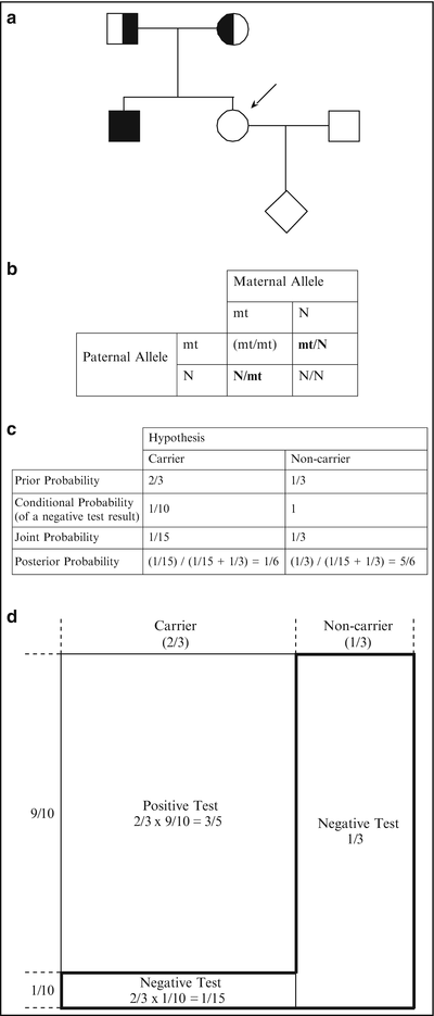
In the second example, information from a test result modifies the prior risk. In the pedigree shown in Fig. 5.2a, the consultand is pregnant with her first child and has a family history of cystic fibrosis (CF; OMIM #219700). CF is caused by mutations in the cystic fibrosis transmembrane conductance regulator gene (CFTR; OMIM #602421). The consultand is an unaffected European Caucasian and her brother died years earlier of complications of CF. She undergoes carrier testing for the 23 mutations recommended by the American College of Medical Genetics (ACMG) CF screening guidelines [11–13], which detects approximately 90 % of disease alleles in European Caucasians. The consultand tests negative for all 23 mutations. What is her carrier risk after testing?


Figure 5.2
(a) Pedigree of a family with an individual affected with CF (see text). Consultand is indicated by an arrow. (b) Possible genotypes of the sibling (consultand in this case) of the affected child prior to genetic testing. The mt/mt genotype (in parentheses) is excluded based on the fact that the consultand is unaffected. Abbreviations: mt mutant, N normal. (c) Bayesian analysis for the consultand in a. (d) Schematic representation of the Bayesian analysis of c (see text)
As in the first example, the two hypotheses are that the consultand is a carrier and that she is a non-carrier. The prior probability that she is a carrier is 2/3. Because the consultand is unaffected, she could not have inherited disease alleles from both parents. Thus, she either inherited a disease allele from her mother or father, or she inherited only normal alleles; in two of these three scenarios she would be a carrier (shown in Fig. 5.2b). The prior probability that the consultand is a non-carrier is 1/3 (Fig. 5.2c).
As in the first example, the conditional probability for each hypothesis is the probability that the subsequent information would occur if we assume that each hypothesis is true. In this example, the subsequent information is that the consultand tests negative for all 23 mutations. Thus, the conditional probabilities are the probability that the consultand would test negative under the assumption (or “condition”) that she is a carrier, and the probability that she would test negative under the assumption (or “condition”) that she is a non-carrier. If we assume that she is a carrier, the probability that she would test negative is 1/10, since the test detects 90 % of European Caucasian disease alleles or carriers. If we assume that she is a non-carrier, the probability that she would test negative approximates 1. Thus, the conditional probabilities in this example are 1/10 and 1 for the carrier and non-carrier hypotheses, respectively (Fig. 5.2c).
As in the first case, the joint probability for each hypothesis is the product of the prior and conditional probabilities for that hypothesis. For the first hypothesis in this example, that the consultand is a carrier, the joint probability is the prior probability that she is a carrier (2/3) multiplied by the conditional probability that a carrier of European Caucasian ancestry would test negative (1/10), or 2/3 × 1/10 = 1/15 (Fig. 5.2c). For the second hypothesis in this example, that the consultand is a non-carrier, the joint probability is the prior probability that she is a non-carrier (1/3) multiplied by the conditional probability that a non-carrier would test negative (1), or 1/3 × 1 = 1/3 (Fig. 5.2c).
Finally, the posterior probability is calculated for each hypothesis by dividing the joint probability for that hypothesis by the sum of all the joint probabilities. In this example, the posterior probability that the consultand is a carrier and tests negative for 23 CF mutations is the joint probability for the first hypothesis (1/15) divided by the sum of the joint probabilities for both hypotheses (1/15 + 1/3 = 2/5), or 1/15 ÷ 2/5 = 1/6 (Fig. 5.2c). The posterior probability that the consultand is a non-carrier and tests negative for 23 CF mutations is the joint probability for the second hypothesis (1/3) divided by the sum of the joint probabilities for both hypotheses (2/5), or 1/3 ÷ 2/5 = 5/6 (Fig. 5.2c).
The preceding example is illustrated graphically in Fig. 5.2d. The total area represents the total prior probabilities. The left 2/3 represents the prior probability that the consultand is a carrier, and the right 1/3 represents the prior probability that the consultand is a non-carrier. Under the hypothesis that the consultand is a carrier, there are two possibilities for the test result: positive or negative. The area of the small rectangle on the lower left comprises 1/10 of the 2/3 carrier region and represents the conditional probability of a normal test result under the hypothesis that the consultand is a carrier. The area of this small rectangle is 1/10 × 2/3 = 1/15 of the total probabilities area and therefore also represents the joint probability that the consultand is a carrier (2/3) and that as a European-Caucasian carrier she would test negative for all 23 mutations (1/10), or 2/3 × 1/10 = 1/15 (Fig. 5.2d).
Under the hypothesis that the consultand is a non-carrier, there is essentially only one possibility for the test result, which is negative. The area of the rectangle that comprises all of the 1/3 non-carrier region represents the conditional probability of a negative test result under the hypothesis that the consultand is a non-carrier. The area of this rectangle is 1/3 of the total area and therefore also represents the joint probability that the consultand is a non-carrier (1/3), and that as a non-carrier she would test negative (~1), or 1/3 × 1 = 1/3. The “reverse-L-shaped” box, which is demarcated by a bold line, represents the sum of the joint probabilities, or 2/5 (=1/3 + 1/15) of the total area.
Because the consultand tested negative, the area of the reverse-L-shaped box represents the only component of the prior probabilities needed to determine the posterior probability that the consultand is a carrier. Taking into account that she tested negative, Bayesian analysis allows us to exclude 3/5 of the prior probability, that portion comprising a positive test result, from consideration. (Note, again, that this explains why the joint probabilities sum to less than 1.) The posterior probability that the consultand is a carrier is therefore the area of the small rectangle at the lower left divided by the area of the reverse-L-shaped box, which represents the only probabilities relevant to the consultand’s risk, or 1/15 ÷ 2/5 = 1/6. Likewise, the posterior probability that the consultand is a non-carrier is the area of the larger rectangle on the right divided by the area of the reverse-L-shaped box, or 1/3 ÷ 2/5 = 5/6.
Simple Bayesian Analyses Generalized: Carrier vs Non-carrier
The preceding Bayesian analyses can be generalized as in Table 5.1. Note that if the correct prior and conditional probabilities can be determined, the rest is simple calculation. Setting up a spreadsheet, as in Table 5.1, facilitates clinical Bayesian analyses.
Table 5.1
Simple Bayesian analyses generalized
Hypothesis | ||
|---|---|---|
1 | 2 | |
Prior probability | A | B = 1 − A |
Conditional probability | C | D |
Joint probability | E = AC | F = BD |
Posterior probability | G = E/(E + F) | H = F/(E + F) |
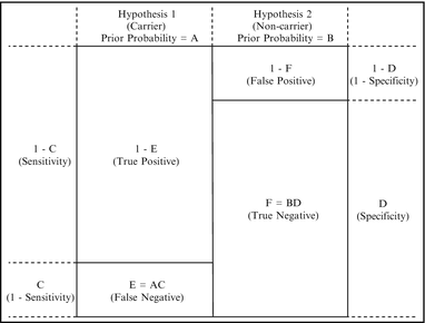
A very common application of Bayesian analysis in molecular pathology is to calculate carrier risk after a negative test result, as in the second example above. The need to calculate carrier risk in this scenario stems from the fact that the sensitivity of most carrier tests is, at present, less than 100 %; therefore, a negative test result decreases, but does not eliminate, carrier risk. Hypothesis 1 in this scenario is that the consultand is a carrier, and Hypothesis 2 is that the consultand is a non-carrier (Table 5.1). The prior carrier probability (“A” in Table 5.1) depends on whether there is a family history, and if so, the relationship of the consultand to the affected family member as shown by the family pedigree. In the absence of a family history, the prior carrier probability is the population carrier risk for that disease. In the case of cystic fibrosis (CF) and some other diseases, the appropriate population risk depends on the ethnicity of the consultand. The conditional probabilities (“C” and “D” in Table 5.1) are one minus the test sensitivity for the carrier hypothesis, and the test specificity for the non-carrier hypothesis, respectively. The remainder of the table is completed through calculation, with the posterior probabilities (“G” and “H” in Table 5.1) representing one minus the negative predictive value, and the negative predictive value, respectively. This is shown schematically in Fig. 5.3.


Figure 5.3
Schematic representation of the generalized Bayesian analysis shown in Table 5.1, for the case of a negative carrier test. The small boxes represent true positive, false positive, true negative, and false negative rates for a particular consultand, i.e., the prior probabilities are influenced by factors such as family history or signs and symptoms, and the sensitivity and specificity of the test are influenced by factors such as ethnicity. For a negative carrier test, the posterior carrier probability (one minus the negative predictive value) is the false negative rate divided by the sum of the false and true negative rates, or E/(E + F).
For illustration, suppose in the second example above (Fig. 5.2) that the consultand’s husband is Ashkenazi Jewish, that he has no family history of CF, and that he tests negative for all 23 mutations in the ACMG screening guidelines panel. What is his carrier risk? The carrier risk in Ashkenazi Jewish populations, and therefore the husband’s prior carrier risk in the absence of a family history, is approximately 1/25 (“A” in Table 5.1). Thus, his prior probability of being a non-carrier is 24/25 (“B” in Table 5.1). The ACMG screening guidelines panel of 23 mutations detects 94 % of CF mutations in Ashkenazi Jewish populations [11–13], so the conditional probability of a negative test, under the hypothesis that he is a carrier, is 6 % = 3/50 (“C” in Table 5.1). Under the hypothesis that he is a non-carrier, the conditional probability of a negative test approximates 1 (“D” in Table 5.1). (This is generally the case in genetic testing, since non-carriers by definition lack mutations in the relevant disease gene and hence, unless there are technical problems, essentially always should test negative.) The Bayesian analysis table for this example is shown in Table 5.2. The joint probabilities (“E” and “F” in Table 5.1) are the products of the prior and conditional probabilities, and the posterior probabilities (“G” and “H” in Table 5.1) derive from each joint probability divided by the sum of the joint probabilities. The husband’s posterior carrier risk after the negative test result is 1/401.
Table 5.2
Bayesian analysis for an Ashkenazi Jewish individual without a family history of CF who tests negative for the ACMG screening guidelines panel of 23 CFTR mutations
Hypothesis | ||
|---|---|---|
Carrier | Non-carrier | |
Prior probability | 1/25 | 24/25 |
Conditional probability (of negative test result) | 3/50 | 1 |
Joint probability | 3/1,250 | 24/25 |
Posterior probability | (3/1,250)/(3/1,250 + 24/25) = 1/401 | (24/25)/(3/1,250 + 24/25) = 400/401 |
What is the risk that the fetus of the mother (consultand) in Fig. 5.2 and the father from Table 5.2 is affected with CF? Prior to testing, the risk was the prior probability that the mother was a carrier (2/3), times the prior probability that the father was a carrier (1/25), times the probability that the fetus would inherit two disease alleles (1/4), or 2/3 × 1/25 × 1/4 = 1/150. After testing, the risk is the posterior probability that the mother is a carrier (1/6), times the posterior probability that the father is a carrier (1/401), times the probability that the fetus would inherit two disease alleles (1/4), or 1/6 × 1/401 × 1/4 ≅ 1/9,600.
Often, testing is performed on additional family members and genetic risks need to be modified accordingly. In the example above, testing of both parents of the mother (consultand) would affect her carrier risk calculations. Detection of mutations in both parents using the same mutation test panel would essentially rule out carrier status for the mother, since we would then know that the sensitivity of the test for the mutations she is at risk of carrying is essentially 100 %. Alternatively, if the test results for the mother’s parents only are positive for one of her parents (for example, her father) and negative for the other parent (her mother), then the sensitivity of the test for the mutations she is at risk of carrying is essentially 50 %. The Bayesian analysis for the mother, modified from Fig. 5.2c, is shown in Table 5.3. The conditional probability of a negative test under the hypothesis that she is a carrier has changed from 1/10 to 1/2, which increases the posterior probability that she is a carrier to 1/2. Taken together with her husband’s carrier risk of 1/401 (Table 5.2), the risk that the fetus is affected with CF can be modified to 1/2 × 1/401 × 1/4 ≅ 1/3,200.
Table 5.3


Bayesian analysis for the consultand in Fig. 5.2a after testing of the parents (see text)
Stay updated, free articles. Join our Telegram channel

Full access? Get Clinical Tree


