approaches the total concentration of enzyme ([E]T) in the assay system. This situation is referred to as tight binding inhibition, and it presents some unique challenges for quantitative assessment of inhibitor potency and for correct assessment of inhibitor SAR.
7.1 Effects of Tight Binding Inhibition on Concentration–Response Data
In the preceding chapters we defined the IC50 as the concentration of inhibitor that results in 50% inhibition of the reaction velocity under a given set of assay conditions. We also defined the term  as the apparent dissociation constant for the enzyme–inhibitor complex, before correction for the inhibition modality-specific influence of substrate concentration relative to KM. In other words, this term is related to the true dissociation constant in different ways, depending on the modality of inhibition displayed by the compound and the ratio [S]/KM used in the activity assay (see Chapter 5). In most cases the terms IC50 and
  are equivalent; however, as we will see now, this is not always the case. Let us consider the following situation: We have screened a chemical library and identified a pharmacophore series that represent competititive inhibitors of our target enzyme. Within this pharmacophore series the most potent hit out of screening is compound A, and this has a
  under our assay conditions of 100 nM. We begin to synthesize analogues of compound A to develop SAR and thus generate four additional compounds in this series, compounds B–E, with increasing affinity for the target enzyme. Let us say that the true value of
  for the five compounds A–E ranges from 100 to 0.01 nM, and that our standard enzyme assay is run at a total enzyme concentration of 50 nM. If we were to perform concentration–response studies for these compounds, we would obtain data similar to what is presented in Figure 7.1. Three observations can be immediately made from viewing the data in Figure 7.1. First, the IC50 values for the more potent inhibitors seem to converge to a common value that is not reflective of the true affinity of the best inhibitors. Second, the data fits for the higher potency inhibitors seem to require Hill coefficients greater than unity for reasonable fits. Third, even with the inclusion of a Hill coefficient >1, the data for the higher affinity compounds is not well described by the simple isotherm equation that we have used until now to describe concentration–response data.
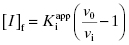
Figure 7.1 Concentration–response plots for a series of compounds displaying  values ranging from 100 to 0.01 nM, when studied in an enzyme assay for which the enzyme concentration is 50 nM. The lines through the data sets represent the best fits to the standard isotherm equation that includes a non-unity Hill coefficient (Equation 5.4). Note that for the more potent inhibitors (where
  ), the data are not well fit by the isotherm equation.
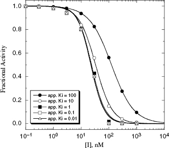
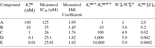
Table 7.1 summarizes the data illustrated in Figure 7.1. We see from this table that the measured IC50 values are not reflective of the  values for the potent compounds; hence the IC50 values here are not a good measure of compound affinity for the target enzyme. Even more disturbing is the fact that the SAR described by measuring the IC50 of the analogue compounds, relative to that of the founder compound (compound A), would suggest that we have not made more than a 5-fold improvement in potency in going from compound A to compound E. Yet the true SAR, reflected by comparison of the relative
  values, indicates that compound E represents a 10,000-fold improvement in target enzyme affinity over compound A. Clearly, reliance on IC50 values in this hypothetical SAR campaign would be terribly misleading. What is the cause of this significant discrepancy between the measured IC50 values and the true
  for this inhibitor series? The answer to this question, as explained in Section 7.2, relates to the concentration of enzyme used in the assay, relative to the
  values of the inhibitors (Easson and Stedman,1936; Henderson, 1972; Cha, 1975; Greco and Hakala, 1979; Copeland et al., 1995).
TABLE 7.1 Measured and True Inhibition Parameters for a Hypothetical Series of Compounds When Measured in an Assay for Which the Enzyme Concentration Is 50 nM
7.2 The IC50 Value Depends on  and [E]T
To explain the results described in Section 7.1, we must consider the relationships between the free and bound forms of the inhibitor under equilibrium conditions. As stated in the preface, our approach throughout this text has been to avoid derivation of mathematical equations and to instead present the final equations that are of practical value in data analysis. In this case, however, it is informative to go through the derivation to understand fully the underlying concepts.
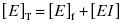
We begin by stating the two mass-balance equations that are germane to enzyme inhibitor interactions:
(7.1) 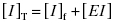
Equation (7.2) reflects a simple bimolecular system of enzyme and inhibitor. It does not account for the fact that in experimental activity measurements there is an additional equilibrium established between the enzyme and the substrate; this will be taken into account below. In the absence of inhibitor [E]T = [E]f. In the presence of inhibitor, the residual velocity that is observed is due to the population of free enzyme, [E]f. Therefore
(7.3) 
or

Equation (7.2) can be recast in terms of mole fractions instead of absolute concentrations by dividing both sides by [E]T:
(7.5) 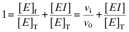
This can be rearranged to yield an equation for [EI]:
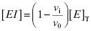
The value of Ki is related to the concentrations of free and bound enzyme and inhibitor as follows:

As stated earlier, the velocity terms are dependent on the concentration of substrate, relative to KM, used in the activity assay. Likewise in an activity assay the free fraction of enzyme is also in equilibrium with the ES complex, and potentially with an ESI complex, depending on the inhibition modality of the compound. To account for this, we must replace the thermodynamic dissociation constant Ki with the experimental value  . Making this change, and substituting Equations (7.4) and (7.6) into Equation (7.7), we obtain (after canceling the common [E]T term in the numerator and denominator)
(7.8) 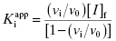
Or, after rearranging,
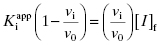
If we multiply both sides of Equation (7.9) by v0/vi and apply the distributive property, we obtain
Combining Equations (7.6) and (7.10) provides an alternative version of the mass-balance equation for the inhibitor:
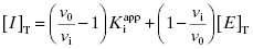
If we set [I]T at the IC50, then, by definition, the values of vi/v0 and v0/vi are fixed to 1/2 and 2.0, respectively. Making these substitutions into Equation (7.11) yields
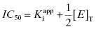
Equation (7.12) defines the influence of both  and enzyme concentration on the measured value of IC50. This equation was first derived by Easson and Stedman (1936), and is correct for all ratios of
  . Strauss and Goldstein (1943) studied the influence of the two terms in Equation (7.12) for different ratios of
  . They divide the treatment of enzyme inhibition data into three distinct zones (Table 7.2). Zone A refers to situations when the ratio
  . Here the 1/2[E]T becomes insignificant relative to
  and the simpler equation
  can be safely used. This is the situation we mainly encountered in the previous chapters of this text. Zone B refers to situations when the ratio
  is between values of 10 and 0.01. In this zone both terms contribute significantly to Equation (7.12), and the full equation must be used in analyzing enzyme inhibition data. Zone C refers to situations when the ratio
  is < 0.01. Here dissociation of the EI complex is negligible, and the inhibitor acts to titrate all of the enzyme molecules in the sample. Hence in this zone the
  value cannot be determined, and IC50 ∼ 1/2[E]T, regardless of the actual value of
  . The data for compounds D and E in Figure 7.1 and Table 7.1 are examples of zone C behavior.
TABLE 7.2 Three Zones of Enzyme–Inhibitor Interactions Defined by Strauss and Goldstein (1943)
| Zone |  | IC50 Equation |
|---|---|---|
| A | >10 |  |
| B | 10–0.01 | 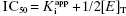 |
| C | <0.01 | IC50 ∼ 1/2[E]T |
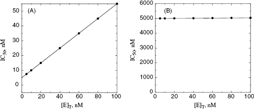
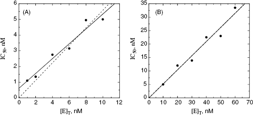
The treatment above provides an explanation for the behavior seen in Figure 7.1 and Table 7.1. It also provides a straightforward method for determining the  value for tight binding inhibitors. By measuring the IC50 at a number of enzyme concentrations, one can construct a plot of IC50 as a function of [E]T and fit these data to a linear equation. As described by Equation (7.12), the y-intercept of such a plot provides an estimate of
  . Figure 7.2 illustrates such plots for two inhibitors measured over a range of enzyme concentrations from 5 to 100 nM. The inhibitor studied in Figure 7.2A has a
  of 5 nM, and over the range of [E]T tested, these experiments fall into Strauss and Goldstein’s zone B. The data are well fit by a linear equation, and the y-intercept faithfully reports the value of
  . The inhibitor in Figure 7.2B has a
  of 5000 nM (i.e., 5 μM), and thus the experiments over the range of [E]T tested fall into Strausss and Goldstein’s zone A. As expected, the IC50 for zone A inhibitors is essentially independent of [E]T and is approximately equivalent to
  , as under these conditions [E]T is such an insignificant fraction of the value of
  .
.
Figure 7.2 Measured IC50 value as a function of total enzyme concentration for (A) an inhibitor displaying a  value of 5 nM, reflecting the behavior of an inhibitor in Strauss and Goldstein’s zone B, and (B) another inhibitor displaying a
  of 5 μM, reflecting the behavior of an inhibitor in Strauss and Goldstein’s zone A. Note that in (B), the line is not horizontal but rather has a slight positive slope due to the minor impact of enzyme concentration on IC50 value under these conditions.
The use of linear plots of IC50 as a function of [E]T is a simple method for determining  for tight binding inhibitors, but there are some limitations to this method. First, it must be recognized that the term [E]T of Equation (7.12), hence of the x-axis of plots such as those in Figure 7.2, does not refer to the total concentration of protein in a sample, but rather to the total concentration of catalytic active sites. Even in a highly purified sample, it can be the case that not all molecules of protein represent active enzyme. Thus reliance on general protein assays, such as Bradford or Lowry dye binding methods (see Copeland, 1994), to determine enzyme concentration is not satisfactory for enzymology studies. This turns out not to be a major issue for the use of linear IC50 versus [E]T plots for the determination of
  . We can generalize Equation (7.12) as follows:
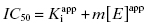
Here m is the slope value and [E]app is the apparent total enzyme concentration, typically estimated from protein assays and other methods (Copeland, 1994). Note from Equation (7.13) that when our estimate of enzyme concentration is incorrect, the slope of the best fit line of IC50 as a function of [E] will not be 1/2, as theoretically expected. Nevertheless, the y-intercept estimate of  is unaffected by inaccuracies in [E]. In fact we can combine Equations (7.12) and (7.13) to provide an accurate determination of [E]T from the slope of plots such as those shown in Figure 7.2. The true value of [E]T is related to the apparent value [E]app as
(7.14) 
or
Thus plots of IC50 as a function of [E]app under conditions of Strauss and Goldstein’s zone B allow one to simultaneously determine the values of  and [E]T using Equations (7.13) and (7.15). Later in this chapter we will see other methods by which tight binding inhibitors can be used to provide accurate determinations of the total concentration of catalytically active enzyme in a sample.
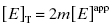
A more severe limitation on the use of IC50 versus [E] plots for the determination of  is one’s ability to accurately determine the y-intercept of a plot for data containing typical levels of experimental error. The ability to differentiate the y-intercept value from zero will depend, in part, on the range of
  values used in the determination of IC50 values. Let us consider an inhibitor for which the value of
  is 0.5 nM. If our enzyme assay provided a robust enough signal to allow us to measure activity at concentrations as low as 1 nM, we might choose to measure the IC50 of the compounds at [E]T = 1, 2, 4, 6, 8, and 10 nM. A plot of IC50 as a function of [E]T for such an experiment is shown in Figure 7.3A; here we have added ±10% random error to our estimates of IC50 for this plot. The best linear fit to these data yields a y-intercept value of 0.6, in good agreement with the true value of
  . The dashed line in this figure is the best fit of the data when the y-intercept is fixed at zero. We can clearly observe that the zero-intercept fit does not describe the experimental data as well as the fit in which the y-intercept is determined as a fitting parameter. On the other hand, suppose that the enzyme assay being employed required a minimum enzyme concentration of 10 nM for acceptable signal over background. Now we might attempt to measure the IC50 of our compound at [E]T = 10, 20, 30, 40, 50, and 60 nM. Again, with ±10% error introduced to the IC50 values, we would obtain a plot as shown in Figure 7.3B. Here a difference in goodness of fit between the fits with the y-intercept fixed at zero and with the y-intercept allowed to float is insignificant. Hence we would have great difficulty obtaining a meaningful estimate of
  from this latter data set. A general rule of thumb is that the highest value of
  used for plots of this type should not exceed 50. Of course, the quality of the data fits, hence the quality of the y-intercept estimate, will depend on the overall quality of the experimentally determined values of IC50 at the various concentrations of enzyme tested.
Figure 7.3 Plots of IC50 as a function of [E]T for an inhibitor of  , measured over a range of enzyme concentrations from 1 to 10 nM (A) and also when measured over a range of enzyme concentrations from 10 to 60 nM. The solid lines in each plot are the best fits of the data to a linear equation. The dashed lines are the best fits of the data to a linear equation for which the y-intercept is fixed at zero.
One final point regarding the influence of [E]T on IC50 that deserves mention is that apparent tight binding behavior is not restricted to situations of very high inherent affinity. At high enough concentrations of enzyme, or other ligand binding proteins, even a modest affinity inhibitor will display tight binding behavior, as this behavior is not determined by  nor [E]T independently but rather by the ratio
  . Hence any time that very high enzyme or protein concentrations are involved, tight binding behavior may be observed. A clinically relevant example of this is the binding of drugs to serum albumin and other serum proteins in systemic circulation. In normal patients the concentration of serum albumin in plasma is approximately 600 μM. At this extremely high concentration of binding protein, even drugs with modest affinity for albumin (e.g., Kd = 1–100 μM) will be driven to high fractional binding. This effect can potentially have a significant influence on the pharmacologically effective dose of a drug, as it is often found that only the albumin-free fraction of drug molecules is available for interactions with their molecular targets (see Chapter 10, Copeland, 2000a, and Rusnak et al., 2004, for examples of the treatment of drug binding to serum proteins).
7.3 Morrison’s Quadratic Equation for Fitting Concentration–Response Data for Tight Binding Inhibitors
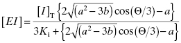
An alternative method for analyzing concentration–response data for tight binding inhibitors was developed by Morrison and coworkers (Morrison, 1969; Williams and Morrison, 1979). This treatment is based on defining the Ki value of an inhibitor, or more generally the Kd value of a ligand, in terms of the free and bound concentrations of enzyme (or protein) and inhibitor (or ligand), without any assumptions regarding the degree of free component depletion due to formation of the binary complex. The derivation of this equation is described in Appendix 2. Here we simply present the final equation that is of practical use:
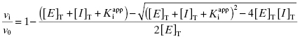
Equation (7.16) is one of two potential solutions to a quadratic equation; it represents the one solution that is physically meaningful. At first glance Equation (7.16) seems hopelessly complicated, but in reality it is relatively easy to write this equation into the library of equations for many commercial curve-fitting programs. In fact several commercial software packages include Morrison’s equation, or a similar equation as part of their standard set of curve-fitting equations (e.g., the software packages Grafit and Prism include such quadratic fitting equations in the standard versions of the curve-fitting software).
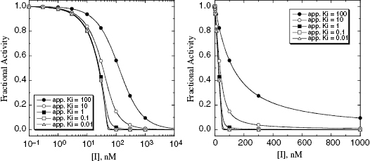
In using Equation (7.16) to fit concentration–response data, the user must experimentally determine the value of vi/v0 at known values of [I]T. The values of  and [E]T can then be allowed to simultaneously float as fitting parameters. Figure 7.4 illustrates the fitting of the data from Figure 7.1 by Equation (7.16). We see that the equation describes well the entire data set for the five inhibitors studied here. The data for this fitting are presented both in semilog scale plots (left panel of Figure 7.4) and in linear scale plots (right panel of Figure 7.4). It is obvious on both scales that the steepness of the response becomes much greater for the more potent inhibitors. This steepness imposes some limits on the range of
  values that can be appropriately analyzed using Morrison’s equation. The optimal conditions for determining
  using this equation have been studied by several authors (Szedlacsek and Duggleby, 1995; Kuzmic et al., 2000a, b; Murphy, 2004), and are summarized below.
Figure 7.4 Concentration–response plots for the data presented in Figure 7.1 fitted to Morrison’s quadratic equation for tight binding inhibitors. The left panel shows the concentration-response behavior on a semilog scale, while the right panel shows the same data when the inhibitor concentration is plotted on a linear scale.
7.3.1 Optimizing Conditions for  Determination Using Morrison’s Equation
Murphy (2004) has reported an in-depth analysis of simulations for various assay conditions using Morrison’s equation for tight binding inhibitors. From these studies several recommendations emerge for optimizing conditions for the determination of  .
.
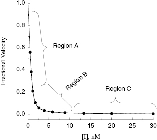
Viewing the fitted data on a linear x-axis scale, Murphy defines three regions of the concentration–response curve (Figure 7.5). Region A is the segment of the curve where the fractional velocity is between 1.0 and about 0.4. Here [I]T < [E]T and the inhibitor is effectively titrating the enzyme concentration in the sample. Data points in this region of the curve are valuable in defining the concentration of enzyme in the sample. In this region of the curve the fractional velocity is a quasi-linear function of inhibitor concentration, and therefore only a few data points are needed to define this region. Murphy suggests limiting the number of data points in this region to ≤3. Region B is what Murphy refers to as the “elbow” region, where the concentration-response data display the most curvature. This occurs in the concentration range where [I]T ∼ [E]T. The data in region B is the most informative for determination of the  value, and therefore experiments should be designed to maximize the number of data points within region B. Region C is where [I]T > [E]T and the values of fractional velocity asymptotically approach zero. It is important to define the steepness of the approach to zero velocity within region C, but as with region A, one need not have more than a few data points (ca. 2 points) to define this portion of the curve.
Figure 7.5 Concentration–response plot for a tight binding enzyme inhibitor, highlighting the three regions of the curve described by Murphy (2004).
Thus Murphy’s analysis suggests that the best experiments for determining  involve inhibitor titrations that maximize the number of inhibitor concentration points in region B of the curve. This is best accomplished with a narrow range of inhibitor concentrations. At the same time one wishes to span a wide enough range of inhibitor concentrations to allow the use of a common titration scheme for the analysis of multiple inhibitors of varying potency. Using 11 inhibitor concentrations for convenient application to microplate-based methods (as described in Chapter 5 and Appendix 3), one finds the best compromise between these opposing requirements comes from using a 1.5-fold inhibitor dilution scheme, as described in Table A3.1 of Appendix 3 (Murphy, 2004).
The next question to be addressed is what the maximum concentration of inhibitor should be at the start of the 1.5-fold dilution series. Murphy suggests starting the dilution series at a concentration of inhibitor equal to 30[E]T (or more correctly 30 times ones best estimate of total enzyme concentration). Simulations suggest that this dilution scheme will provide adequate data points within region B for inhibitors with potencies ranging from 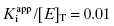 to 10.
7.3.2 Limits on  Determinations
Use of Morrison’s quadratic equation, together with Murphy’s recommended dilution scheme, will allow accurate estimates of  as low as 100-fold below the total enzyme concentration. Based on Murphy’s simulations, the most accurate determination of
  is obtained for inhibitor titrations performed at
  (Murphy, 2004).
Of course, the accuracy of these determinations depends on the quality of the experimental data used to construct the concentration–response plots; significant data scatter will erode the accuracy of the fitting parameter estimates.
Murphy’s analysis of simulated data suggest that one can obtain accurate determinations of both  and [E]T simultaneously from fitting of the data to Morrison’s equation. He makes the point that allowing both parameters to be determined by fitting provides superior estimates of
  than can be obtained by fixing [E]T to an inaccurate value. While this may be true, it is my experience that in the presence of reasonable levels of experimental data scatter, allowing both
  and [E]T to float in the fitting routine can lead to physically meaningless estimates of [E]T and also to inaccuracies in the determination of
  . Thus, in my view, the best method for determining
  for tight binding inhibitors is to apply Morrison’s equation with [E]T fixed at a value that has been experimentally determined by an accurate method. It is critical that the reader appreciate the importance of this point. The value of [E]T used in conjunction with Morrison’s equation must reflect accurately the concentration of active enzyme molecules, and not merely the concentration of total protein. Fixing the value of [E]T in the equation incorrectly can have serious consequences on the resulting determinations of
  . Fortunately the use of tight binding inhibitors themselves provide a highly accurate method for determining the true concentration of active enzyme in a sample. This method will be presented at the end of this chapter.
7.3.3 Use of a Cubic Equation When Both Substrate and Inhibitor Are Tight Binding
Because they are catalytic, most enzymes do not display tight binding behavior toward their substrates, as this would be counterproductive to efficient catalysis (Fersht, 1999; Copeland, 2000b). However, occasionally one encounters an enzyme for which the KS for substrate, or the Kd for an activating cofactor, is very low. This creates a difficulty in experimental interpretation of tight binding inhibitor data as both ligands—the inhibitor and the substrate—display tight binding behavior. Wang (1995) has presented a treatment for this type of situation in the context of competitive ligand binding to receptor molecules. For a competitive, tight binding enzyme inhibitor, the concentration of binary EI complex is defined by the following cubic equation.
where
(7.18) 
(7.19) 
(7.20) 
(7.21) 
Again, this situation is rarely encountered in analysis of enzyme inhibitors when using activity asssays. However, use of Equation (7.17) may be required in situations where one uses an equilibrium binding measurement to determine the ability of a test compound to displace a known tight binding inhibitor from the target enzyme. This is commonly encountered, for example, in fluorescence polarization assays in which a fluorescently labeled ligand (i.e., an enzyme inhibitor) is used as a primary ligand, and test compounds are studied for their ability to displace the fluorescent ligand from the enzyme or receptor molecule (see Copeland, 2000, and references therein, for a discussion of these methods).
7.4 Determining Modality for Tight Binding Enzyme Inhibitors
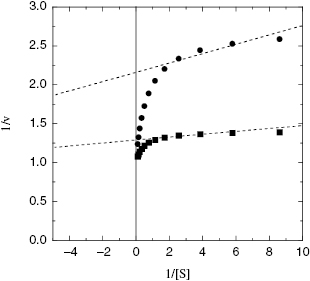
Because enzyme binding significantly depletes the population of free inhibitor molecules at concentrations where tight binding inhibitors are effective, the classical steady state equations for initial velocity are no longer applicable. Morrison and coworkers (Morrison, 1969; Williams and Morrison, 1979) have derived alternative equations to describe the steady state velocity of enzymes in the presence of tight binding inhibitors. For our purposes the most critical point to glean from this analysis is that the traditional graphical methods for determining inhibitor modality, particularly the use of double reciprocal plots, can be very misleading when tight binding behavior is in play. For all inhibition modalities the double reciprocal plots for tight binding inhibitors are nonlinear. For example, Figure 7.6 illustrates the double reciprocal plot for a tight binding competitive inhibitor. We note that the nonlinear plots converge to a common y-intercept value, as would be expected for a competitive mode of inhibition. However, the nonlinearity of the double reciprocal plot is only apparent at the higher substrate concentrations. If one were to perform this type of analysis over a less complete range of substrate concentrations (e.g., if the substrate solubility limited ones ability to make measurements at high substrate concentrations), one could easily misinterpret the data as conforming to linear double reciprocal lines that converge beyond the y-axis. In other words, the pattern of lines seen in this situation would be most consistent with the classical behavior for noncompetitive inhibition. There are a number of examples in the literature of tight binding competitive inhibitors that, for the reasons just described, have been misinterpreted as noncompetitive inhibitors (e.g., see Turner et al., 1983). In fact, over a limited range of [S]/KM values, the double reciprocal plots for tight binding inhibitors display the expected behavior for classical noncompetitive inhibition, regardless of the true inhibition modality of the compound.
Figure 7.6 Double reciprocal plot for a tight binding competitive enzyme inhibitor, demonstrating the curvature of such plots. The dashed lines represent an attempt to fit the data at lower substrate concentrations to linear equations. This highlights how double reciprocal plots for tight binding inhibitors can be misleading, especially when data are collected only over a limited range of substrate concentrations.
Stay updated, free articles. Join our Telegram channel

Full access? Get Clinical Tree


