6.1 Determining kobs: The Rate Constant for Onset of Inhibition
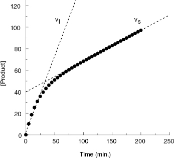
The hallmark of slow binding inhibition is that the degree of inhibition at a fixed concentration of compound will vary over time, as equilibrium is slowly established between the free and enzyme-bound forms of the compound. Often the establishment of enzyme–inhibitor equilibrium is manifested over the time course of the enzyme activity assay, and this leads to a curvature of the reaction progress curve over a time scale where the uninhibited reaction progress curve is linear. We saw this behavior in Figure 5.10, for a reaction initiated by simultaneous addition of a slow binding inhibitor and substrate to the target enzyme. In Figure 6.1 we again illustrate a typical progress curve in the presence of a slow binding inhibitor. We see that the progress curve here reflects two distinct velocities for the reaction. In the early time points, before the enzyme–inhibitor equilibrium is established fully, the progress curve is linear, and the velocity derived from the slope of this portion of the curve is defined as the initial velocity, vi. The value of vi may be identical to that of the uninhibited reaction, or may vary with inhibitor concentration, depending on the specific mechanism of inhibition. Toward the end of the progress curve, the product concentration again appears to track linearly with time, but the velocity measured from the slope of this portion of the progress curve is much less than the initial velocity. The velocity measured near the end of the progress curve reflects the steady state velocity achieved after equilibration of the enzyme and inhibitor. This velocity is given the symbol vs. In the time points between these two linear phases, the progress plot displays significant curvature, as the system transitions from the initial to the steady state velocity. For any particular reaction at fixed concentrations of enzyme, substrate, and slow binding inhibitor, we can fit the progress curve by an equation that contains terms for the initial and steady state velocities, and for the rate constant for conversion from the initial velocity phase to the steady state velocity phase, kobs:
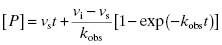
Figure 6.1 Typical progress curve for an enzyme reaction in the presence of a slow binding inhibitor. The initial (vi) and steady state (vs) velocities are defined by the slope values in the early and late stages of the progress curve, respectively, as indicated by the dashed lines.
If the inhibitor potency is such that the concentration of inhibitor required to affect significant, time-dependent inhibition is similar to the concentration of enzyme, then one must account for the tight binding nature of the inhibition (discussed further in Chapter 7). In this case Equation (6.1) is modified as follows:
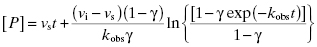
where
Fitting of a progress curve, such as that shown in Figure 6.1 to either Equation (6.1) or (6.2) allows one to obtain an estimate of kobs, vi, and vs at a specific concentration of compound.
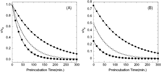
In some cases the establishment of enzyme–inhibitor equilibrium is much slower than the time course of the enzyme activity assay. In these cases the reaction progress curves may appear linear, and the detection of a time-dependence of inhibition will depend on measurements of steady state velocity before and after a long preincubation of the enzyme with inhibitor (or ES with inhibitor in the case of a bisubstrate reaction for which the slow binding inhibitor is uncompetitive with one of the substrates; vide infra) prior to initiation of reaction with substrate(s). If very slow binding inhibition is occurring, one should observe a difference in the velocity or % inhibition realized before and after pre-incubation. When this is seen, the steady state velocity can be measured over a range of pre-incubation times. The results of such an experiment are illustrated in Figure 6.2. We see from this figure that the steady state velocity falls off exponentially with preincubation time. Data such as that shown in Figure 6.2 can thus be fit to the following equation:
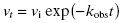
where vt is the measured steady state velocity after preincubation time t, and vi is the steady state velocity at preincubation time = 0. The value of vi is similar to the steady state velocity in the absence of inhibitor when there is not a rapid phase of inhibition preceding the slower step (Figure 6.2 A). On the other hand, when there is a rapid phase of inhibition prior to the slower step, the value of vi will vary with inhibitor concentration (Figure 6.2 B). By these methods one can again obtain an estimate of kobs at varying concentrations of inhibitor.
Figure 6.2 Effect of preincubation time with inhibitor on the steady state velocity of an enzymatic reaction for a very slow binding inhibitor. (A) Preincubation time dependence of velocity in the presence of a slow binding inhibitor that conforms to the single-step binding mechanism of scheme B of Figure 6.3. (B) Preincubation time dependence of velocity in the presence of a slow binding inhibitor that conforms to the two-step binding mechanism of scheme C of Figure 6.3. Note that in panel B both the initial velocity (y-intercept values) and steady state velocity are affected by the presence of inhibitor in a concentration-dependent fashion.
6.2 Mechanisms of Slow Binding Inhibition
The common mechanisms of slow binding inhibition are summarized in Figure 6.3. Scheme A of this figure shows the uninhibited enzyme reaction in which ES complex formation and dissociation are governed by the second-order association rate constant k1 (i.e., kon) and the first-order dissociation rate constant k2 (i.e., koff). Scheme B illustrates a simple reversible equilibrium between the enzyme and inhibitor governed by association and dissociation rate constants k3 and k4, respectively. This is identical to the expected behavior for any reversible inhibitor (see Chapter 3), except that here the values of k3 and/or k4 are much smaller, leading to the slow realization of inhibition. A number of physical origins can be envisaged for an inherently slow rate of binding or of dissociation. For example, inhibitor binding at an enzyme active site might require the slow expulsion of a tightly bound water molecule. Also very high affinity interactions, such as that seen for transition state analogues, can manifest slow dissociation rates of the EI complex.
Figure 6.3 Mechanisms for slow binding inhibition of enzymatic reactions. (A) The enzyme reaction in the absence of inhibitor. (B) A single-step binding mechanism for which the association rate (determined by k3) or dissociation rate (determined by k4) or both are inherently slow. (C) A two-step binding mechanism for which the first step is simple, rapid equilibrium binding of inhibitor to enzyme to form an encounter complex (EI) and the second step is a slow isomerization of the enzyme to form a higher affinity complex, E*I. This mechanism is referred to as the induced-fit mechanism. (D) A two-step binding mechanism for which the first step is slow isomerization of the free enzyme to an inhibitor-binding conformation (E*) and the second step is rapid equilibrium binding of the inhibitor to this new conformational state of the enzyme. This mechanism is referred to as the conformational selection mechanism. (E) Covalent modification of the enzyme by an affinity label or a mechanism-based inhibitor. The intact inhibitory species (XI) first binds reversibly to the enzyme to form an encounter complex (EI). Then a slower chemical step occurs leading to covalent attachment of the inhibitor to a catalytically essential group on the enzyme and release of the leaving group X. These and other mechanisms for covalent inactivation of enzymes will be discussed in Chapter 9.
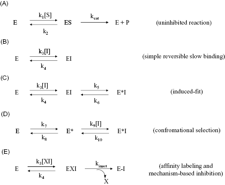
In scheme C of Figure 6.3 the induced-fit mechanism of slow binding is illustrated. This is perhaps the most common mechanism of slow binding for drug-like enzyme inhibitors, as discussed further in Chapter 8. Here the inhibitor encounters the enzyme in an initial conformation that leads to formation of a binary complex of modest affinity. It is generally assumed that this initial encounter complex forms under rapid equilibrium conditions, similar to the simple, reversible inhibitors discussed in Chapter 3 (see Sculley et al., 1996, for a treatment of mechanisms such as scheme C when this rapid equilibrium assumption does not hold). Hence the affinity of the initial encounter complex, EI, is defined by the ratio of the rate constants k4/k3, which is equal to the Ki of the encounter complex. Subsequent to initial complex formation, the enzyme undergoes an isomerization step (k5), which is much slower than the reversible steps associated with the encounter complex. This isomerization results in much higher affinity binding between the inhibitor and the new enzyme conformational state, represented by the symbol E*. The reverse isomerization step that returns E*I to the initial encounter complex EI is governed by the first-order rate constant k6. Thus formation of the final E*I complex is rate-limited by k5 and dissociation of ligand from the E*I complex is rate-limited by the reverse isomerization step, governed by k6. The true affinity of the inhibitor is therefore not realized until formation of the E*I complex; hence any measure of slow-binding inhibitor affinity for this mechanism must take into account the values of Ki, k5, and k6 (vide infra).
In principle, there are two additional mechanisms for slow binding behavior that involve isomerization of one of the binding partners. The first is a mechanism in which the inhibitor slowly isomerizes between two forms in solution, with only one of the isomers being capable of high-affinity interactions with the enzyme. This mechanism is not represented in Figure 6.3 as it is not commonly encountered with small molecular weight drugs. The second additional mechanism (scheme D) is referred to as the conformational selection mechanism. Here the free enzyme slowly isomerizes in solution between two alternative forms, E and E*, and only one of these forms (E*) goes on to rapidly combine with inhibitor to form the binary complex E*I. It would seem that this latter mechanism is similar to what is shown in scheme C of Figure 6.3, as both mechanisms result in the same final species, E*I. However, the velocity equation for the mechanism involving isomerization of the free enzyme results in the value of kobs decreasing as a function of increasing inhibitor concentration. As we will see below, this behavior allows the experimenter to clearly distinguish the latter mechanism from that shown in scheme C. An example of a binding reaction involving isomerization of the free enzyme is the binding of aromatic substrates to the serine protease chymotrypsin. In solution chymotrypsin slowly isomerizes between two alternative conformational states, only one of which is capable of binding and processing aromatic substrates (Fersht, 1999). Like the inhibitor isomerization mechanism discussed above, the free enzyme isomerization mechanism is rarely encountered with small molecular weight inhibitors (but see Chapter 8). Hence we will not consider either of these alternative mechanisms further; the interested reader can learn more about these mechanisms in Chapter 8, in the review by Morrison (1982) and in Duggleby et al. (1982).
The fourth mechanism that results in slow binding behavior is covalent inactivation of the enzyme by affinity labeling or mechanism-based inhibition (Scheme E, Figure 6.3). These forms of irreversible inhibition will be the subject of Chapter 9, and we will defer further discussion of these mechanisms until that chapter.
6.3 Determination of Mechanism and Assessment of True Affinity
In this section we focus on differentiating slow binding inhibition due to the mechanisms shown in schemes B and C of Figure 6.3.
To distinguish between simple, reversible slow binding (scheme B) and an induced-fit mechanism (scheme C), one can examine the dependence of kobs on inhibitor concentration. If the slow onset of inhibition merely reflects inherently slow binding and/or dissociation, then the term kobs in Equations (6.1) and (6.2) will depend only on the association and dissociation rate constants k3 and k4 as follows:

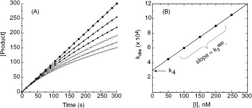
This is a linear equation, and we can thus expect kobs to track linearly with inhibitor concentration for an inhibitor conforming to the mechanism of scheme B. As illustrated in Figure 6.4, a replot of kobs as a function of [I] will yield a straight line with slope equal to k3 and y-intercept equal to k4. It should be noted that in such an experiment the measured value of k3 is an apparent value as this association rate constant may be affected by the concentration of substrate used in the experiment, depending on the inhibition modality of the compound (vide infra). Hence the apparent value of Ki ( ) for an inhibitor of this type can be calculated from the ratio of k4/k3(apparent), which is equivalent to the ratio of the y-intercept/slope from the linear fit of the data plotted as in Figure 6.4 B. This apparent Ki value can then be converted to a true Ki by consideration of the inhibition modality of the compound, as will be discussed below.
Figure 6.4 (A) Progress curves for an enzymatic reaction in the presence of increasing concentrations of a slow binding inhibitor that conforms to the single-step binding mechanism of scheme B of Figure 6.3. (B) A replot of kobs for the progress curves in (A) as a function of inhibitor concentration. The linear fit of the data in panel B provides estimates of the kinetic rate constants k4 (from the y-intercept) and of the apparent value of k3 (from the slope), as these rate constants are defined in scheme B of Figure 6.3.
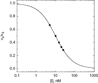
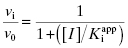
In the mechanism illustrated by scheme B, significant inhibition is only realized after equilibrium is achieved. Hence the value of vi (in Equations 6.1 and 6.2) would not be expected to vary with inhibitor concentration, and should in fact be similar to the initial velocity value in the absence of inhibitor (i.e., vi = v0, where v0 is the steady state velocity in the absence of inhibitor). This invariance of vi with inhibitor concentration is a distinguishing feature of the mechanism summarized in scheme B (Morrison, 1982). The value of vs, on the other hand, should vary with inhibitor concentration according to a standard isotherm equation (Figure 6.5). Thus the IC50 (which is equivalent to  ) of a slow binding inhibitor that conforms to the mechanism of scheme B can be determined from a plot of vs/v0 as a function of [I].
Figure 6.5 Concentration–response plot of inhibition by a slow binding inhibitor that conforms to scheme B of Figure 6.3. The progress curves of Figure 6.4A were fitted to Equation (6.1). The values of vs thus obtained were used together with the velocity of the uninhibited reaction (v0) to calculate the fractional activity (vs/v0) at each inhibitor concentration. The value of  is then obtained as the midpoint (i.e., the IC50) of the isotherm curve, by fitting the data as described by Equation (6.8).
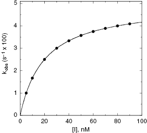
For the induced-fit enzyme isomerization mechanism illustrated in scheme C of Figure 6.3, there are two steps involved in formation of the final enzyme–inhibitor complex: an initial encounter complex that forms under rapid equilibrium conditions and the slower subsequent isomerization of the enzyme leading to the high-affinity complex. The value of kobs for this mechanism is a saturable function of [I], conforming to the following equation:
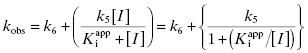
where  is the apparent value of the Ki for the initial encounter complex (i.e., k4/k3(apparent)). Equation (6.6) is similar in form to the Michaelis-Menten equation that we described in Chapter 2. Thus a plot of kobs as a function of [I] for this mechanism yields a rectangular hyperbola, as illustrated in Figure 6.6. Here the y-intercept is nonzero and is equal to the rate constant k6. The maximum value of kobs (kmax) is equal to the sum k6 + k5, and the concentration of inhibitor yielding a half-maximal value of kobs is equal to
  . Again,
  can be converted into the true value of Ki for the initial inhibitor encounter complex if the modality of inhibition is known (vide infra). Thus, by fitting data such as that shown in Figure 6.6 to Equation (6.6), one can obtain estimates of the forward and reverse enzyme isomerization rate constants (k5 and k6, respectively) and of the apparent dissociation constant for the initial inhibitor encounter complex (
 ). The true affinity of an inhibitor that conforms to this mechanism is defined by the dissociation constant for the final high-affinity conformation of the enzyme–inhibitor complex; this can be calculated as follows:
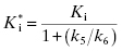
Figure 6.6 (A) Progress curves for an enzymatic reaction in the presence of increasing concentrations of a slow binding inhibitor that conforms to the two-step binding mechanism of scheme C of Figure 6.3. (B) A replot of kobs for the progress curves in (A) as a function of inhibitor concentration. The data in this replot are a hyperbolic function of inhibitor concentration, as described by Equation (6.6). The y-intercept, from curve fitting of these data to Equation (6.6), provides an estimate of k6, while the maximum value of kobs (kmax), at infinite inhibitor concentration, reflects the sum of k5 and k6.
Thus, by analysis of the effects of inhibitor concentration on kobs, we can obtain estimates of the affinity of the inhibitor for both the initial and final conformational states of the enzyme.
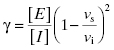
In a two-step induced-fit mechanism, as in scheme C, the affinity of the inhibitor encounter complex and the affinity of the final E*I complex are reflected in the diminutions of vi and of vs, respectively, that result from increasing concentrations of inhibitor. The apparent values of Ki and of  can therefore be obtained as the IC50s of the isotherms for vi/v0 and for vs/v0, respectively, as illustrated in Figure 6.7:
and
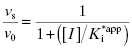
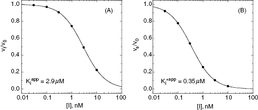
Figure 6.7 Concentration–response plots for the initial (A) and final (B) inhibited states of an enzyme reaction inhibited by a slow binding inhibitor that conforms to the mechanism of scheme C of Figure 6.3. The values of vi and vs at each inhibitor concentration were obtained by fitting the data in Figure 6.6A to Equation (6.1). These were then used to calculate the fractional velocity (vi/v0 in panel A and vs/v0 in panel B), and the data in panels A and B were fit to Equations (6.8) and (6.9) to obtain estimates of  and
and  , respectively.
Note that for very slow binding inhibitors that are studied by varying preincubation time, the fits of the exponential decay curves to Equation (6.4) provide values for both vi and kobs for each inhibitor concentration. The values of vi at each inhibitor concentration represent the y-intercepts of the best fit to Equation (6.4), and these can be used in conjunction with Equation (6.8) to obtain an independent estimate of  .
.
The form of Equation (6.7) reveals an interesting aspect of slow binding inhibiton due to enzyme isomerization. A slow forward isomerization rate is insufficient to result in slow binding behavior. The reverse isomerization rate must also be slow, and in fact must be significantly slower that the forward isomerization rate. If this were not the case, there would be no accumulation of the E*I conformation at equilibrium. As the value of k6 becomes >> k5, the denominator of Equation (6.7) approaches unity. Hence the value of  approaches Ki, and one therefore does not observe any time-dependent behavior.
On the other hand, when  , the concentration of inhibitor required to observe slow binding inhibition would be much less than the value of Ki for the inhibitor encounter complex. When, for example, the inhibitor concentration is limited, due to solubility or other factors, and therefore cannot be titrated above the value of Ki, the steady state concentration of the EI encounter complex will be kinetically insignificant. Under these conditions it can be shown (see Copeland, 2000) that Equation (6.6) reduces to
Equation (6.10) is a linear function with 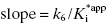 and y-intercept = k6. Hence a plot of kobs as a function of [I] will yield the same straight-line relationship as seen for the mechanism of scheme B. Therefore the observation of a linear relationship between kobs and [I] cannot unambiguously be taken as evidence of a one-step slow binding mechanism.
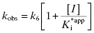
When k6 is very small, there is very little return of the system from E*I to EI and subsequently to E + I on any reasonable measurement time scale. In this case the inhibitor has the appearance of an irreversible inhibitor and the value of vs approaches zero at all inhibitor concentrations (see Chapter 9). Inhibitors displaying this behavior are referred to as a slow, tight binding inhibitors because the very low value of k6 in turn drives the term  to very low values. When k6 is very small, it is difficult to distinguish its value from zero. Hence a plot of kobs as a function of [I] will remain hyperbolic, but the y-intercept will now be close to the origin, and the maximum value of kobs will be equal to k5 (Figure 6.8). The term k6 in Equation (6.6) can thus be ignored, and the kinetics of inhibition are therefore indistinguishable from true irreversible inactivation of the enzyme (see Chapter 9). If k6 is extremely low, it may not be possible to distinguish between irreversible inactivation and slow, extremely tight binding inhibition by kinetic methods alone (see Chapters 5, 8, and 9 for other ways to distinguish between these mechanisms). However, in cases where k6 is small, but not extremely small, one can use two types of experiments to attempt to measure the value of k6. First, it can be shown through algebraic manipulations of Equations (6.6) through (6.9), that the value of kobs is a function of vi, vs, and k6:
(6.11) 
or

Figure 6.8 Replot of kobs as a function of inhibitor concentration for a slow binding inhibitor that conforms to the mechanism of scheme C of Figure 6.3 when the value of k6 is too small to estimate from the y-intercept of the data fit.
Thus, if the reaction progress curve can be followed for a long enough time, under conditions where the unihibited enzyme remains stable, one may be able to measure a small, but nonzero, value for vs. Combining this value with vi and kobs would allow one to determine k6 from Equation (6.12).
Second, one can use the type of rapid dilution experiments described in Chapter 5 to estimate the value of this rate constant. According to Morrison (1982) slow, tight binding inhibitors are almost always active-site directed, hence competitive with respect to substrate (but see below). Let us therefore say that we are dealing with a slow binding competitive inhibitor for which the value of k6 is too small to distinguish from zero by fitting the kobs versus [I] plot as in Figure 6.8. We could incubate the inhibitor and enzyme together at high concentrations as described in Chapter 5 and then rapidly dilute the pre-formed E*I complex into assay buffer. We would then obtain a progress curve similar to that shown in Figure 5.9C. A curvilinear progress curve for recovery of enzymatic activity as in Figure 5.9C can be fit to an equation like Equation (6.2), except that now the initial and steady state velocities would reflect the E*I and EI states, respectively. The kobs value obtained from such an experiment would depend on inhibitor concentration according to Equation (6.6). However, if we were to make a large dilution of the E*I pre-formed complex (so that the final concentration of inhibitor was very low) into an assay buffer containing saturating concentrations of substrate (i.e., [S]/KM > 5), the very high substrate concentration, together with the very low final inhibitor concentration, would effectively compete out any rebinding of inhibitor to the free enzyme. The value of  for a competitive inhibitor is Ki(1 + [S]/KM) according to the Cheng-Prusoff relationship (see Chapter 5). As [S]/KM becomes large and [I]/Ki becomes small after dilution, the second term in Equation (6.6) approaches zero. Hence under these conditions the value of kobs provides a reasonable approximation of the value of k6. In this way one can obtain a reasonable estimate of the rate constant for reversal of isomerization. In situations where the magnitude of k4 is similar to that of k6, the kobs value obtained by rapid dilution will reflect the combined influence of k4, k5, and k6 (kobs = k4 k6/(k4 + k5 + k6); see Chapter 8). Even under these non-ideal conditions, the value of kobs will reflect the rate of the overall inhibitor dissociation process (koff). Since this rate constant reflects the rate limiting step(s) for reactivation of the enzyme, one can use this rate constant to define the dissociation half-life for slow binding inhibitors (see Appendix 1):
(6.13) 
or
(6.14) 
Note that instead of plotting product formed as a function of time after rapid dilution (as in Figure 5.9), some researchers instead plot percent of activity recovered with time after dilution, referencing activity to a control sample of enzyme that is not exposed to inhibitor prior to dilution (i.e., 100% activity control). In this manner, the percent activity increases in a pseudo-first order manner as a function of time after dilution (Narjes et al., 2000). Hence, the value of kobs can be determined in this case from a simple first-order equation:
(6.15) 
See Chapter 8 for a more complete discussion of the importance of the dissociative half-life, and the related residence time (1/k6 or 1/kobs), of enzyme inhibitor complexes.
6.3.1 Potential Clincial Advantages of Slow Off-Rate Inhibitors
In some cases the duration of pharmacodynamic activity is directly related to the residence time of the inhibitor on its target enzyme (i.e., the duration of inhibition), and this is defined by the dissociation half-life for compounds that function as slow, tight binding inhibitors (discussed further in Chapter 8). The determination of the dissociation half-life, together with the estimate of true target affinity represented by  , can therefore be of great value in defining the appropriate dosing concentrations and intervals for in vivo compound assessment. In principle, a compound displaying a very low value of k6, hence a very long dissociation half-life, could confer a significant clinical advantage over rapidly reversible inhibitors. Once such a compound is bound to its target, the activity of the target enzyme is effectively shut down for a significant time period (especially if the rate of new enzyme synthesis by the cell is too slow to sustain viability; that is, new enzyme synthesis cannot overcome inhibition of existing enzyme). The concentration of compound in systemic circulation need only be high, relative to
  , long enough for the inhibitor to encounter the target enzyme. Hence the Cmax can be reduced to reflect the high affinity of the E*I complex and the pharmacokinetic half-life required for efficacy can also be significantly reduced. The reduced time of high compound levels in systemic circulation would in turn reduce the potential for off-target interactions of the compound, potentially reducing the likelihood of off-target toxicity. Thus compounds that display slow off rates from their targets can, in some cases, offer important advantages in clinical medicine (see also Chapters 7 and 8).
Stay updated, free articles. Join our Telegram channel

Full access? Get Clinical Tree


