4.1.2 Total, Background, and Specific Signal
In the preceding section we defined the total signal and background signal as they relate to construction of a calibration or standard curve for assay development. In the context of calibration curves made with genuine samples of analyte, it is usually reasonable to assume that the background signal is constant. However, during an actual enzyme reaction, the background signal may not be constant for any of a number of reasons. For example, suppose we wish to follow the enzyme-catalyzed hydrolysis of a peptide by following fluorescence signal. The N- and C- termini of the peptide can be modified to incorporate a fluorophore and a fluorescence quencher, respectively, such that fluorescence intensity is significantly augmented upon cleavage of the peptide by the protease. One could thus measure fluorescence intensity as a function of time after initiating the enzyme reaction (by addition of enzyme or substrate to the reaction mixture) to generate a reaction progress curve, such as that illustrated in Figure 4.2. However, control experiments of the substrate in reaction buffer, without the enzyme, may demonstrate that there is some modest level of non-enzymatic, background hydrolysis of the substrate. This background hydrolysis reaction would lead to a nonconstant background signal that increases with reaction time, as also illustrated in Figure 4.2. The signal that is specific to the course of the enzymatic reaction is thus the difference between the total signal and the background signal at each individual time point; this difference is referred to as the specific signal (Θs) and is also sometimes referred to as the specific signal window:
(4.1) 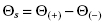
Figure 4.2 Illustration of total (filled squares), background (open circles), and specific (closed circles) signal associated with the progress curve of an enzyme-catalyzed reaction. The specific signal is calculated by subtracting background signal from total signal at each time point.
There is a common misconception among some members of the screening community that the signal-to-background ratio (Θ(+)/Θ(−)) is an appropriate measure of enzyme reaction progress (or velocity), but a moment’s reflection will demonstrate that this is clearly incorrect. The signal-to-background ratio is a useful metric of assay performance (Macarron and Hertzberg, 2002), but it is a dimensionless metric, as one is dividing signal, molarity, or molarity per unit time by the identical unit. On the other hand, specific signal (Θs) retains the correct dimensionality of the signal. Thus, all measurements of enzymatic activity should be reported as specific signal (i.e., total signal minus background) prior to conversion of specific signal into molarity units by use of the calibration curve.
Let us walk through an example to illustrate these concepts. We will again use the example of a protease assay of peptide hydrolysis for our illustration. Whenever a proteolytic enzyme (e.g., protease) acts on a fluorogenic peptide substrate, it produces two products in equal molar amounts, an N-terminal cleavage product and a C-terminal cleavage product. Let us say that we have synthesized genuine samples of the N- and C-terminal cleave product peptides, with the appropriate fluorophore and quencher appended to the appropriate termini (see above). We can create a calibration curve by serial dilution into assay buffer of a concentrated solution of equal concentrations of the two product peptides. Let us say that we determine that within the linear dynamic range, the fluorescence signal corresponds to 1000 fluorescence units (FU) per micromolar (μM) product. Now let us say that we set up a reaction solution containing 50 μM substrate peptide, in appropriate buffer, and we initiate the reaction by adding enzyme to a final concentration of 0.05 μM. Let us say that the signal increases linearly with time over 30 minutes from an initial value of 10 FU to a final value of 3060 FU. Over this same time course, a control reaction without enzyme also shows a linear increase in signal intensity from an initial value of 10 FU to a final value of 60 FU. Subtracting the background signal for each time point, we find that the specific signal has changed over the 30 minute time course from 0 FU to 3000 FU. Stated otherwise, the velocity of the reaction over this time course is 100 FU per minute. Using the conversion factor of 1000 FU = 1 μM from the calibration curve, we can then calculate that the velocity of the reaction is 0.1 μM/minute and that the total product produced over the course of the 30 minute time course is 3.0 μM. This means that we have produced 3 μM product from 50 μM substrate in the course of the 30 minute enzyme reaction, or in other words, we have converted 6% of the starting substrate to product.
The importance of measuring specific signal and converting this to molarity of substrate or product is that it allows the researcher a way to keep quantitative account of reaction progress during the course of steady state assay conditions. Such quantitative bookkeeping is critical to ensure that the enzyme assay is working appropriately for inhibitor discovery. For example, a well-behaved enzyme assay under steady state conditions should reflect multiple turnover events of the enzyme. Hence, it is expected that the concentration of substrate consumed and of product produced will be in great excess of the total concentration of enzyme used in the reaction. Likewise, at all time points in the course of the enzymatic reaction, there should be conservation of mass between the substrate and product of the reaction, such that the sum of the molar concentrations of substrate and product at any time point must be equal to the starting molar concentration of substrate (these comments refer to a specific substrate and its cognate product in the case of multi-substrate enzyme reactions):
(4.2) 
where [S]0 is the starting molar concentration of substrate, [S]t and[P]t are the molar concentrations of substrate, and product at time = t. If either of the above conditions are not fulfilled, the assay under consideration must be considered suspect and most likely will be inappropriate for use in inhibitor screening.
4.1.3 Defining Inhibition, Signal Robustness, and Hit Criteria
The goal of most screening assays for enzyme targets is to identify compounds that act as inhibitors of enzymatic activity. To identify and compare inhibitory compounds, we must first define a metric that reflects the ability of a fixed concentration of compound to reduce the activity of the target enzyme. The most commonly used metric for this purpose is the percent inhibition, which can be defined as follows. The velocity of the enzyme reaction in the absence of inhibitory compound is defined from the slope of a plot of specific signal (or molarity) as a function of time (i.e., after correction for any time-dependent background signal, as described in the preceding section), and is symbolized by v0. Likewise, the velocity in the presence of a fixed concentration of inhibitor ([I]) is also determined as the slope from a plot of specific signal as a function of time, and this is symbolized by vi. The fractional activity remaining in the presence of a fixed concentration of inhibitor is given by the ratio vi/v0. The limits of vi/v0 are 1.0 at [I] = 0 and 0 at [I] = ∞ (assuming complete inhibition; see Chapter 3). Thus, the fractional inhibition seen at a fixed concentration of compound is related to the fractional activity remaining as 1 − (vi/v0). The percent inhibition is thus calculated as the fractional inhibition multiplied by 100:
It is clear from Equation (4.3) that one’s ability to accurately measure reaction velocity, hence inhibition, is dependent on the strength of the signal due to the catalysis and relative to any background signal. However, in any real assay the signal due to catalysis and that due to background are not absolute constants, but instead each displays some variability, depending on the assay and detection method details (vide supra). Figure 4.3 illustrates the type of variability in catalytic signal and background that one might observe for a well-behaved assay. Both the catalytic signal and the background can be described by a Gaussian distribution centered around a mean value with the distribution width being defined by a standard deviation for each measurement. Clearly, one’s ability to distinguish a true change in catalytic signal will depend not only on the mean values of catalytic and background signals but also on the magnitudes of their respective standard deviations; that is, one’s ability to distinguish real changes in catalytic signal, due to the presence of an inhibitor, can be compromised by significant variability in the catalytic signal or in the background, or both. Zhang et al. (1999) have derived a simple statistical test by which to judge the assay quality based on the concepts above. The statistical measure they derived is referred to as Z′ and is defined as follows:
(4.4) 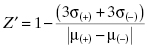
where again μ(+) and σ(+) are the mean and standard deviation for the catalytic signal, respectively, μ(−) and σ(−) are the mean and standard deviation for the background signal, respectively, and the denominator term is the absolute value of the difference in the means of the two measures. The maximum value of Z′ is unity for a perfect assay in which both the signal and background standard deviations are zero. The lower the value of Z′, the greater the signal (catalytic or background) variability is, hence the less discrimination power the assay has. In practice, it has been generally found that assays that afford a Z′ value ≥0.5 are acceptable for high throughput library screening. The Z′ statistic is a general measure of assay robustness that can be applied to any enzymatic or other assay; it is not restricted to use for HTS purposes.
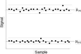
With an appropriately robust assay one can measure the ability of library components to inhibit the enzyme of interest, and rank-order the “hits” in terms of the % inhibition that each produces at a fixed, common concentration. Typically library components are tested at fixed concentrations of 1 to 30 μM for HTS. For a library of reasonable size (anywhere from 10,000 compounds for academic libraries up to >1 million compounds for large pharmaceutical companies) and chemical diversity, one expects that the vast majority of library components will not affect the target enzyme. The number of library components that are true inhibitors of a target enzyme is expected to be very small, typically ≤1% for an unbiased, diverse library. Thus we would expect that the majority of library components would display a Gaussian distribution of % Inhibition, centered around a value close to zero and with a breadth determine by the standard deviation. With such a distribution of results, how would one rationally classify a compound as a hit? In other words, what constitutes a significant amount of inhibition that would allow us to designate a particular library component as having scored positive as an inhibitor of our target enzyme? The answer to this question depends on the degree of statistical confidence that one requires. Generally, for a Gaussian distribution, a component displaying a value that differs from the mean value by ≥2 standard deviations is considered to be statistically different with a 95% confidence limit, while a value ≥3 standard deviations from the mean is considered to be statistically different with a 99.73% confidence limit (Motulsky, 1995). Many screening groups use the more stringent criterion of ≥3 standard deviations from the library mean value to designate library components as hits. For example, let us say that the mean % inhibition for an unbiased library is 3.1% with a standard deviation of 10.6%. The mean plus 3 standard deviations would put our 99.73% confidence limit at 34.9% inhibition. By this measure any library component that inhibited the target enzyme by ≥34.9% would be deemed a hit (Figure 4.4). One could decide to use this statistically sound criterion for hit declaration, but could also decide to increase or decrease the stringency, depending on the hit rate (i.e., the number of compounds that would be deemed a hit) for a particular screen. If one is concerned that the number of hits will be too low, one could reduce the stringency by accepting as hits, compounds that were only 2 standard deviations from the mean (i.e., at the 95% confidence limit), accepting the increased risks associated with this decision. In contrast, if one is concerned that the number of hits will be too high to be tractable, one could use a higher, somewhat arbitrary cutoff of 50% inhibition in our hypothetical screen. Alternatively, one could reduce the number of hits by retaining the 99.73% confidence limit cutoff, but screening at a lower concentration of inhibitor (e.g., switching from a screen at 10 μM compound to one at 1 μM compound).
Figure 4.4 Histogram of typical screening results for a hypothetical enzyme assay. The hits are designated as those compounds that displayed a % inhibition equal to or greater than three standard deviation units above the mean.
4.2 Measuring Initial Velocity
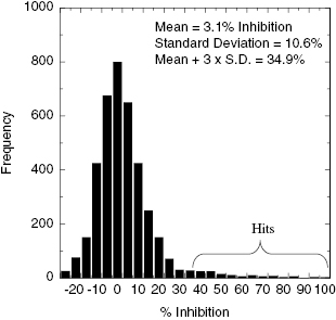
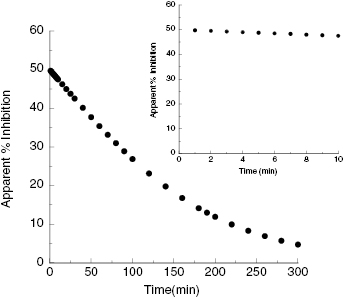
In Chapter 2 we described the typical product progress curve for a well-behaved enzyme and introduced the concept of initial velocity. In assays designed to quantify the ability of a test compound to inhibit the target enzyme, it is critical to restrict the assay time to the initial velocity phase of the reaction. The reason for this can be illustrated with the following example. Suppose that we were to measure the full progress curve for an enzyme reaction in the absence of inhibitor and also in the presence of an amount of inhibitor that reduced the reaction velocity by half. Assuming that the background is zero for our hypothetical assay, we can expect the value of vi/v0 to be 0.5; hence from Equation (4.3), the % inhibition can be expected to be 50%. At this concentration of a reversible enzyme inhibitor, we have (averaged over time) half of the enzyme population bound by inhibitor, hence inactive, and half of the population of enzyme molecules free of inhibitor, and hence still active. In this situation the enzyme molecules that are not bound by inhibitor will continue to turn over substrate to produce product, albeit at a slower overall rate (because the effective concentration of active enzyme has been reduced by half). Therefore product production will still continue until a significant proportion of substrate has been utilized. Figure 4.5 illustrates the expected progress curves for our hypothetical enzyme assay in the presence and absence of inhibitor. We can see from this figure that the effect of the inhibitor is less apparent as the progress curve proceeds. During the early time points (i.e., during the initial velocity phase) the effect of the inhibitor is most apparent, as illustrated by the inset of Figure 4.5. Later, however, the apparent % inhibition is diminished because of the continuing accumulation of product with time, both in the presence and absence of inhibitor. This point is highlighted in Figure 4.6 where the apparent % inhibition is plotted as a function of time for the two progress curves shown in Figure 4.5. As illustrated in the inset of Figure 4.6, only during the initial velocity phase (up to about 10–20% substrate depletion) is the % inhibition relatively constant and close to the true value; a similar analysis of the effects of the degree of substrate conversion on the apparent IC50 value for enzyme inhibitors was recently presented by Wu et al. (2003). Therefore there are two good reasons for ensuring that HTS assays are measured during the initial velocity phase of enzymatic reactions. First, the initial velocity is the best measure of enzyme reaction rate, and the use of this parameter makes subsequent analysis of reaction mechanism and inhibition modality most straightforward, as described in Chapters 2 and 3. Second, the initial velocity phase of the reaction is the most sensitive to the influence of reversible inhibitors (as illustrated above). Hence assays that run under initial velocity conditions provide the most effective means of detecting inhibitory molecules during library screening (Copeland, 2003). Exceptions to this generalization can, however, occur in situations where the forward reaction catalyzed by the enzyme is rapidly reversed, either by the back reaction or by nonenzymatic side reactions. This unusual situation has been discussed by Jordan et al. (2001).
Figure 4.5 Product progress curves for an enzyme-catalyzed reaction in the absence (closed circles) and presence (open circles) of an inhibitor at a concentration that reduces the reaction rate by 50%. Inset: The initial velocity phase of these progress curves.
Figure 4.6 Calculated % inhibition as a function of reaction time from the progress curves shown in Figure 4.5. Note that as the reaction continues past the initial velocity phase (shown in the inset), the apparent % inhibition is dramatically diminished.
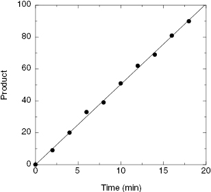
4.2.1 End-Point and Kinetic Readouts
The initial velocity of reaction is defined by the slope of a linear plot of product (or substrate) concentration as a function of time (Chapter 2), and we have just discussed the importance of measuring enzymatic activity during this initial velocity phase of the reaction. The best measure of initial velocity is thus obtained by continuous measurement of product formation or substrate disappearance with time over a convenient portion of the intial velocity phase. However, continuous monitoring of assay signal is not always practical. Copeland (2000) has described three types of assay readouts for measuring reaction velocity: continuous assays, discontinuous assays, and end-point assays. The meaning of continuous assay is obvious, and this applies to systems where the signal can be monitored throughout the reaction time course. Spectroscopic assays, for example assays based on absorbance or fluorescence signals, can often be set up in the laboratory as continuous assays. Discontinuous assay refers to a situation where the assay must be stopped, or quenched, prior to signal detection. One determines the initial velocity then by stopping aliquots of the reaction mixture at various times to produce a plot of the product formation or substrate disappearance as a function of these discrete time points. A common example of a discontinuous assay is the measurement of 33P incorporation into a peptidic substrate of a protein kinase, which is done by detecting radioactivity after binding to a filter (Figure 4.7). In such assays one typically uses a reaction mixture of sufficient volume so that convenient size samples can be removed, quenched, and assayed at evenly spaced time points throughout the reaction. The third readout method is referred to as an end-point assay, and it is identical to the discontinous assay method, except that here a single time point is chosen at which to detect signal generation (sometimes this is modified to use two time points, an initial reading at time = 0 and the end-point reading at time = t). The advantages of the end-point readout are obviously reduced monitoring, reduced instrumentation time, and general convenience. These advantages are particularly important to robot-based HTS methods. There are, however, some caveats that must be recognized in the use of end-point assays.
Figure 4.7 Example of a reaction progress curve obtained by discontinuous measurement of 33P incorportation into a peptide substrate of a kinase. Each data point represents a measurement made at a discrete time point after initiation of the reaction with γ-33P-ATP.
The underlying assumption in any end-point assay is that the time point measured is well within the initial velocity phase of the reaction, so that product formation or substrate disappearance is a linear function of time. If this is true, then the velocity equation can be reduce to a simple ratio of the change in signal over the change in time:

where ΔΘ is the change in signal that occurs during the time interval Δt. If the signal at time zero is negligible and constant, Equation (4.5) can be simplified even further to the simple ratio Θ/t. Thus, if the time of reading is fixed, the signal intensity becomes directly proportional to velocity and can be used without further transformation as a readout of reaction progress. This works well as long as the underlying assumption of linear reaction velocity is true. In my experience, however, one cannot make this assumption without experimental verification. Even in situations where one has established the duration of the initial velocity phase in the laboratory, it is not always safe to assume that this will remain the same when the assay is re-formatted for robotic HTS applications. Hence end-point assays are very convenient for HTS purposes, and can be used safely and effectively. However, this requires the prior rigorous determination of the reaction progress curve under the exact assay conditions to be used for HTS.
For both discontinuous and end-point assays, another underlying assumption is that the conditions used to stop, or quench, the reaction lead to an instantaneous and permanent halt of signal production. Again, this is an important assumption that requires experimental verification. If the reaction is slowed down, but not truly stopped by the quenching conditions, serious problems with signal reproducibility can be encountered. Copeland (2000) has discussed a variety of methods for quenching enzymatic reactions, and for verifying these stopping conditions.
4.2.2 Effect of Enzyme Concentration
If we were to fix the substrate concentration at which an enzyme assay is performed, we could combine Equations (2.12) and (2.13) to obtain the simple equation

where λ = kcat[S]/([S] + Km). Hence our expectation from Equation (4.6) is that the initial velocity should track linearly with enzyme concentration at any fixed substrate concentration. This is exactly the situation we would like to have in quantitative screening for inhibitors of enzymatic activity. In a situation where velocity tracks linearly with enzyme concentration, a 50% reduction in active enzyme molecules (caused by 50% occupancy of enzyme–inhibitor complex) will produce a 50% reduction in the observed velocity. It is critical that the diminution of reaction velocity quantitatively correlate with the formation of the enzyme–inhibitor complex if we are to correctly rank-order compound potency from screening assays. Equation (4.6) seems to reassure us that this is not an issue for enzymatic reactions. While most enzymes display this expected behavior, in practice deviations can be encountered.
Figure 4.8 illustates the correlation between reaction velocity and enzyme concentration for a poorly behaved assay. At low concentrations the observed velocity is less than expected, based on a simple linear correlation with enzyme concentration. This can occur for several reasons. First, the signal intensity of the assay detection method may be inadequate at these low enzyme concentration to provide an accurate assessment of velocity. Second, at very low enzyme concentrations, enzyme loss or denaturation can occur, especially due to adsorption of enzyme molecules to vessel surfaces (see Copeland, 1994 and 2000, for more detailed discussions). Last, some enzymes require dimer or higher order oligomeric structures to form an active enzyme species. A pharmacologically relevant example of this is the HIV protease, which is synthesized by the virus as a 99 amino acid monomer. The active protease, however, is formed by dimerization of the protein, each monomer providing one of the two essential active site aspartic acid residues of the enzyme. Hence the active site of catalysis is not formed until protein dimerization occurs. Formation of the HIV protease dimer is an equilibrium process which is disfavored at very low enzyme concentrations (see Morelock et al., 1996, for a discussion of the impact of the HIV protease monomer-dimer equilibrium on the proper analysis of inhibition data). Thus, at a low concentration, enzymes like the HIV protease might show a discontinuity in the velocity versus [E] plot because of the underlying monomer-dimer equilibrium that is taking place.
Figure 4.8 Reaction velocity as a function of enzyme concentration for a non-ideal enzymatic activity assay. Note the deviations from the expected linear relationship at low and at high enzyme concentration.
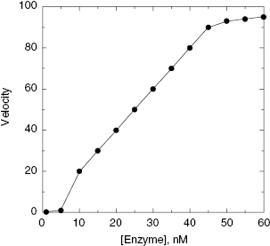
Deviations from linearity at high enzyme concentrations can also have multiple origins. The most common reason for an apparent deviation from linearity here is that the high enzyme concentrations speed up the reaction so much that one inadvertently moves out of the initial velocity phase of the reaction, and into a phase of greater substrate depletion. This, as seen in Figure 4.6, has the effect of slowing down the apparent velocity as the steady state conditions no longer hold. Also one must consider the linear dynamic range of detection methods in determining assay conditions. If the signal produced by product formation exceeds the dynamic range of ones detection method, the apparent velocity will be diminished. High enzyme concentrations can be one cause of this problem. This can be especially problematic for fluorescence-based detection methods. As the concentration of fluorescent product increases, limitations in detection of the emitted photons, such as inner filter effects, can occur. This and other sources of error due to detection limitations have been discussed in Copeland (2000). Finally, some enzymes are only fully active in a monomer or low molecular weight oligomeric form. As the concentration of enzyme increases one can drive the formation of higher order oligomeric species which may have diminished catalytic activity. This again would lead to the type of deviations from linearity illustrated in Figure 4.8 at high enzyme concentration.
Thus the best approach for HTS purposes is to experimentally determine the effect of enzyme titration on the observed reaction velocity, and to then choose to run the assay at an enzyme concentration well within the linear portion of the curve (as in Figure 4.8). Again, the other details of the assay conditions can affect the enzyme titration curve, so this experiment must be performed under the exact assay conditions that are to be used for library screening.
4.2.3 Other Factors Affecting Initial Velocity
Enzymatic reactions are influenced by a variety of solution conditions that must be well controlled in HTS assays. Buffer components, pH, ionic strength, solvent polarity, viscosity, and temperature can all influence the initial velocity and the interactions of enzymes with substrate and inhibitor molecules. Space does not permit a comprehensive discussion of these factors, but a more detailed presentation can be found in the text by Copeland (2000). Here we simply make the recommendation that all of these solution conditions be optimized in the course of assay development. It is worth noting that there can be differences in optimal conditions for enzyme stability and enzyme activity. For example, the initial velocity may be greatest at 37°C and pH 5.0, but one may find that the enzyme denatures during the course of the assay time under these conditions. In situations like this one must experimentally determine the best compromise between reaction rate and protein stability. Again, a more detailed discussion of this issue, and methods for diagnosing enzyme denaturation during reaction can be found in Copeland (2000).
It is almost always the case that enzymes are most active under the solution conditions that best match the physiological conditions experienced by the enzyme (see Table 4.1 for typical physiological conditions for mammalian cell cytosol). There are, however, exceptions to this generalization. Sometimes one will find that the laboratory conditions that maximize catalytic activity are different from one’s expectation of physiological conditions. In such cases a careful judgment must be made about what conditions to use for screening purposes. Whenever possible, my bias is to screen at conditions that most closely match the physiological conditions. We saw, for example, in Chapter 3 how substrate KM and inhibitor potency were significantly affected by changing assay conditions to reflect physiological ionic strength in the case of the kinesin motor protein KSP (see Table 3.10). However, this statement assumes that one truly understands the cellular environment that is experienced by the target enzyme. Subcellular compartmentalization and other factors can generate conditions that are quite different from what we generally think of as “physiological.” For example, if asked, most biologists would quote pH 7.4 as being close to physiological pH. However, this is based on averaged measurements of blood plasma and other tissue samples. The average pH experienced by a gastric enzyme would be far lower, as would that of enzymes compartmentalized within endosomes and lysosomes of cells. Thus some attention must be paid to learning as much as possible about the environment in which the target enzyme conducts its biological function.
TABLE 4.1 Some Typical Values of Physiological Conditions for Mammalian Cell Cytosol
Source: Lodish, H. F., Berk, A., Kaiser, C. A., Krieger, M., Scott, M. P., Bretscher, A., and Ploegh, H. (2007), Molecular Cell Biology, 6th ed., W. H. Freeman, New York; Periaswamy et al. (1991), Biochemistry 30: 11836–11841.
| Parameter | Value |
|---|---|
| pH | 7.3–7.5 |
| Ionic strength | ∼150 mM |
| Cation composition | |
| Potassium | 139 mM |
| Sodium | 12 mM |
| Magnesium | 0.8 mM |
| Calcium | <0.0002 mM |
| Water content | 70% |
| Viscosity | 1.2–1.4 cPa |
a cP = centipoise.
In some cases one’s best guess at physiological conditions does not support sufficient catalytic activity to make a screening assay feasible. In this situation one has no choice but to compromise in favor of more optimal laboratory conditions. Nevertheless, one should attempt, whenever possible, to come as close as feasible to assay conditions that reflect the physiological context in which the target enzyme operates.
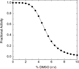
To be pharmacologically active, enzyme inhibitors must conform to certain physicochemical parameters, and this usually includes a certain degree of hydrophobicity in the inhibitor molecule. Hence drug-like enzyme inhibitors often have limited solubility in aqueous solution. To assay the inhibitory potential of such compounds, one must usually prepare a stock solution of the compound in an aprotic solvent. The inhibitor is then added to the aqueous enzyme reaction mixture in the form of a concentrated stock solution. The tolerance of enzymes for the addition of nonaqueous solvents varies from enzyme to enzyme. For this reason it is critical that one determine the concentration of nonaqueous solvent that is tolerated without significant diminution of activity for the particular target enzyme, under the exact conditions to be used in screening. The most common solvent used for inhibitor dissolution is dimethyl sulfoxide (DMSO). Before initiating a screen in which library components will be added to the assay reaction mixture in the form of a DMSO stock solution, one should determine the effect of DMSO concentration on the activity of the target enzyme. A simple DMSO titration, as depicted in Figure 4.9, will guide the researcher as to the maximum tolerated concentration of solvent that can be used. Based the results of such a titration, one should then fix the concentration of DMSO in all enzyme reactions for screening, including all controls (e.g., reactions run in the absence of inhibitor), at a concentration high enough to effect adequate compound solubility but low enough to not significantly attenuate enzymatic activity. In rare cases target enzymes display a very low tolerance for DMSO as a co-solvent. In these cases alternative solvents must be considered.
Figure 4.9 Example of the effect of dimethyl sulfoxide (DMSO) concentration on the initial velocity of an enzyme-catalyzed reaction.
The discussion above was concerned with the effects of solution conditions on enzyme activity, hence reaction velocity. Equally important for the purpose of assay design is the influence of specific solution conditions on the detection method being used. This latter topic is beyond the scope of the present text. Nevertheless, this is an important issue for screening scientists whose job is often to balance the needs of biochemical rigor and assay practicality in development of an HTS assay. An excellent discussion of these more assay design-specific issues can be found in the review by Macarron and Hertzberg (2002).
4.3 Balanced Assay Conditions
The goal of library screening should be to identify as diverse a group of lead compounds as possible, and as stated before, lead diversity should be viewed both in terms of diversity of chemical structure and diversity of inhibition modality (Copeland, 2003). We have already stated several times that it is almost impossible to predict what inhibition modality will provide the best cellular and in vivo efficacy. Dogmatic arguments that lead to a priori predictions of what will work best in a biological context more often than not reflect an incomplete understanding of cellular physiology and of the myriad interactions among macromolecules that occur in living systems. Likewise arguments based on historic precedence of “what has already been proven to work” only hold until someone else demonstrates a new way of solving the problem. Hence, whenever possible, one should bring forward, in parallel, optimized compounds of several modalities for biological testing and allow the biology to define the best candidates for further consideration. To achieve this goal, HTS assays must be conducted under conditions that balance the opportunities to identify inhibitors of all modalities that may be present in a compound library.
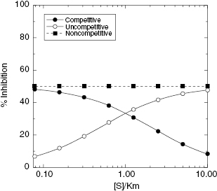
In Chapter 3 we saw that inhibitors of different modalities respond differently to the concentration of substrate used in an enzymatic reaction. Recall that the apparent affinity of the free enzyme for substrate was diminished in the presence of a competitive inhibitor, and vice versa, the apparent affinity of a competitive inhibitor could be abrogated at high substrate concentrations. On the other hand, the apparent affinity of an uncompetitive inhibitor was seen to be augmented by high substrate concentrations. Let us again consider the velocity equations for competitive, noncompetitive and uncompetitive inhibition that were presented in Chapter 3. In the context of library screening it is typical for the concentration of potential inhibitors to be fixed at a single concentration, typically between 1 and 30 μM. Let us say that we set up a screening assay in which library components will be individually tested as inhibitors at a fixed concentration of 10 μM. Let us further say that within this screening library are attractive lead compounds that behave as competitive, noncompetitive (α = 1) and uncompetitive inhibitors of our target enzyme, each with an inhibitor dissociation constant of 10 μM. How will the concentration of substrate used in our screening assay affect our ability to discovery these various inhibitors within our library? Using the velocity equations presented in Chapter 3, and Equation (4.3) of this chapter, we can calculate the % inhibition observed as a function of substrate concentration, relative to KM, for the three inhibitor types just described. The results of these calculations are summarized in Figure 4.10. For the noncompetitive inhibitor, we see that the observed % inhibition is unaffected by the [S]/KM value chosen for screening. This is true because we have fixed the value of α at unity. For noncompetitive inhibitors with α ≠ 1, we would see some change in % inhibition as the substrate concentration was changed. In the case of competitive and uncompetitive inhibition, however, we see dramatic changes in the observed % inhibition with titration of the substrate. Lower values of the ratio [S]/KM increase the apparent inhibition caused by a fixed concentration of competitive inhibitor; hence low substrate concentrations favor the identification of competitive inhibitors in HTS assays. In contrast, the apparent inhibition caused by a fixed concentration of an uncompetitive inhibitor is greatest at the higher concentrations of substrate, so that these conditions favor the identification of uncompetitive inhibitors in HTS assays.
Figure 4.10 Observed % inhibition as a function of [S]/KM for competitive (closed circles), noncompetitive (α = 1, closed squares) and uncompetitive (open circles) inhibition. Conditions used for simulation: Ki = αKi = [I]. Note that the [S]/KM axis is plotted on a logarithmic scale for clarity.
Stay updated, free articles. Join our Telegram channel

Full access? Get Clinical Tree


