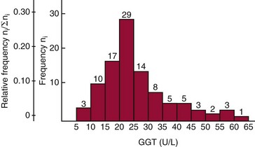
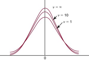
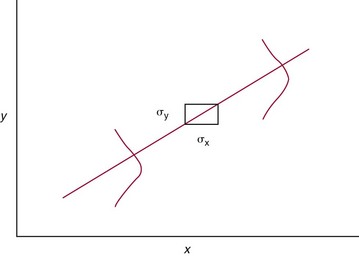
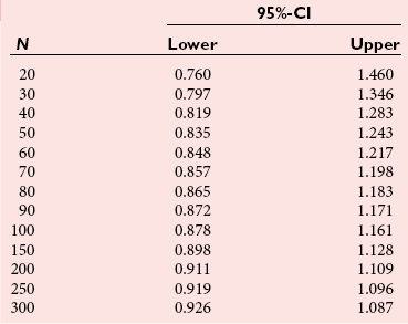
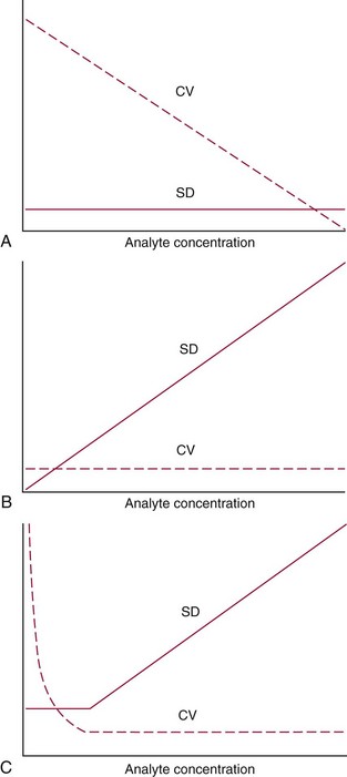
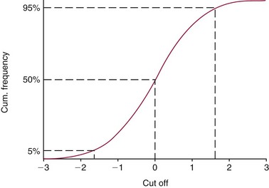
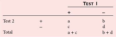
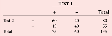
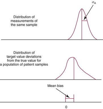
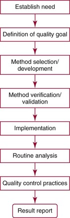
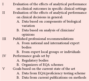
Chapter 2 The introduction of new or revised methods is a common occurrence in the clinical laboratory. Method selection and evaluation are key steps in the process of implementing new methods (Figure 2-1). A new or revised method must be selected carefully and its performance evaluated thoroughly in the laboratory before it is adopted for routine use. Establishment of a new method may also involve evaluation of the features of the automated analyzer on which the method will be implemented. Figure 2-1 A flow diagram that illustrates the process of introducing a new method into routine use. When a new method is to be introduced to the routine clinical laboratory, a series of evaluations are commonly conducted. Assay imprecision is estimated and comparison of the new assay versus an existing method or versus an external comparative method is undertaken. The allowable measurement range is assessed with estimation of the lower and upper limits of quantification. Interferences and carryover are evaluated when relevant. Depending on the situation, a limited verification of manufacturer claims may be all that is necessary, or, in the case of a newly developed method in a research context, a full validation must be carried out. Subsequent subsections provide details for these procedures. With regard to evaluation of reference intervals or medical decision limits, please see Chapter 5. Method evaluation in the clinical laboratory is influenced strongly by guidelines.26,105,106 The Clinical and Laboratory Standards Institute [CLSI, formerly National Committee for Clinical Laboratory Standards (NCCLS)] has published a series of consensus protocols11–19 for clinical chemistry laboratories and manufacturers to follow when evaluating methods (see the CLSI website at http://www.clsi.org). The International Organization for Standardization (ISO) has also developed several documents related to method evaluation.43–50 In addition, meeting laboratory accreditation requirements has become an important aspect in the method selection and/or evaluation process with accrediting agencies placing increased focus on the importance of total quality management and assessment of trueness and precision of laboratory measurements. An accompanying trend has been the emergence of an international nomenclature to standardize the terminology used for characterizing method performance. This chapter presents an overview of considerations in the method selection process, followed by sections on method evaluation and method comparison. The latter two sections focus on graphical and statistical tools that are used to aid in the method evaluation process; examples of the application of these tools are provided, and current terminology within the area is summarized. The selection of appropriate methods for clinical laboratory assays is a vital part of rendering optimal patient care, and advances in patient care are frequently based on the use of new or improved laboratory tests. Ascertainment of what is necessary clinically from a laboratory test is the first step in selecting a candidate method. Key parameters, such as desired turnaround time and necessary clinical utility for an assay, are often derived by discussions between laboratorians and clinicians. When new diagnostic assays are introduced, reliable estimates of clinical sensitivity and specificity must be obtained from the literature or by conducting a clinical outcome study (see Chapter 4). With established analytes, a common scenario is the replacement of an older, labor-intensive method with a new, automated assay that is more economical in daily use. In these situations, consideration must be given to whether the candidate method has sufficient precision, accuracy, analytical measurement range, and freedom from interference to provide clinically useful results (see Figure 2-1). In evaluation of the performance characteristics of a candidate method, (1) precision, (2) accuracy (trueness), (3) analytical range, (4) detection limit, and (5) analytical specificity are of prime importance. The sections in this chapter on method evaluation and comparison contain detailed outlines of these concepts and their assessment. Estimated performance parameters for a method are then related to quality goals that ensure acceptable medical use of the test results (see section on “Analytical Goals”). From a practical point of view, the “ruggedness” of the method in routine use is of importance and reliable performance when used by different operators and with different batches of reagents over long time periods is essential. 1. Principle of the assay, with original references. 2. Detailed protocol for performing the test. 3. Composition of reagents and reference materials, the quantities provided, and their storage requirements (e.g., space, temperature, light, humidity restrictions) applicable both before and after the original containers are opened. 4. Stability of reagents and reference materials (e.g., their shelf life). 5. Technologist time and required skills. 6. Possible hazards and appropriate safety precautions according to relevant guidelines and legislation. 7. Type, quantity, and disposal of waste generated. 8. Specimen requirements (e.g., conditions for collection and transportation, specimen volume requirements, the necessity for anticoagulants and preservatives, necessary storage conditions). 9. Reference interval of the method, including information on how it was derived, typical values obtained in health and disease, and the necessity of determining a reference interval for one’s own institution (see Chapter 5 for details on how to generate a reference interval). 10. Instrumental requirements and limitations. 12. Computer platforms and interfacing with the laboratory information system. 13. Availability of technical support, supplies, and service. 1. Does the laboratory possess the necessary measuring equipment? If not, is there sufficient space for a new instrument? 2. Does the projected workload match with the capacity of a new instrument? 3. Is the test repertoire of a new instrument sufficient? 4. What is the method and frequency of calibration? 5. Is staffing of the laboratory sufficient for the new technology? 6. If training the entire staff in a new technique is required, is such training worth the possible benefits? 7. How frequently will quality control samples be run? 8. What materials will be used to ensure quality control? 9. What approach will be used with the method for proficiency testing? 10. What is the estimated cost of performing an assay using the proposed method, including the costs of calibrators, quality control specimens, and technologists’ time? A graphical device for displaying a large set of data is the frequency distribution, also called a histogram. Figure 2-2 shows a frequency distribution displaying the results of serum gamma-glutamyltransferase (GGT) measurements of 100 apparently healthy 20- to 29-year-old men. The frequency distribution is constructed by dividing the measurement scale into cells of equal width, counting the number, ni, of values that fall within each cell, and drawing a rectangle above each cell whose area (and height, because the cell widths are all equal) is proportional to ni. In this example, the selected cells were 5 to 9, 10 to 14, 15 to 19, 20 to 24, 25 to 29, and so on, with 60 to 64 being the last cell. The ordinate axis of the frequency distribution gives the number of values falling within each cell. When this number is divided by the total number of values in the data set, the relative frequency in each cell is obtained. Often, the position of the value for an individual within a distribution of values is useful medically. The nonparametric approach can be used to determine directly the percentile of a given subject. Having ranked N subjects according to their values, the n-percentile, Percn, may be estimated as the value of the [N(n/100) + 0.5] ordered observation.23 In the case of a noninteger value, interpolation is carried out between neighbor values. The 50-percentile is the median of the distribution. Consider again the frequency distribution in Figure 2-2. In addition to the general location and spread of the GGT determinations, other useful information can be easily extracted from this frequency distribution. For instance, 96% (96 of 100) of the determinations are less than 55 U/L, and 91% (91 of 100) are greater than or equal to 10 but less than 50 U/L. Because the cell interval is 5 U/L in this example, statements such as these can be made only to the nearest 5 U/L. A larger sample would allow a smaller cell interval and more refined statements. For a sufficiently large sample, the cell interval can be made so small that the frequency distribution can be approximated by a continuous, smooth curve, similar to that shown in Figure 2-3. In fact, if the sample is large enough, we can consider this a close representation of the true population frequency distribution. In general, the functional form of the population frequency distribution curve of a variable x is denoted by f(x). The population frequency distribution allows us to make probability statements about the GGT of a randomly selected member of the population of healthy 20- to 29-year-old men. For example, the probability Pr(x > xa) that the GGT value x of a randomly selected 20- to 29-year-old healthy man is greater than some particular value xa is equal to the area under the population frequency distribution to the right of xa. If xa = 58, then from Figure 2-3, Pr(x > 58) = 0.05. Similarly, the probability Pr(xa < x < xb) that x is greater than xa but less than xb is equal to the area under the population frequency distribution between xa and xb. For example, if xa = 9 and xb = 58, then from Figure 2-3, Pr(9 < x < 58) = 0.90. Because the population frequency distribution provides all information related to probabilities of a randomly selected member of the population, it is called the probability distribution of the population. Although the true probability distribution is never exactly known in practice, it can be approximated with a large sample of observations. where xi is an individual measurement and N is the number of sample measurements. The Gaussian probability distribution, illustrated in Figure 2-4, is of fundamental importance in statistics for several reasons. As mentioned earlier, a particular analytical value x will not usually be equal to the true value µ of the specimen being measured. Rather, associated with this particular value x will be a particular measurement error ε = x − µ, which is the result of many contributing sources of error. Pure measurement errors tend to follow a probability distribution similar to that shown in Figure 2-4, where the errors are symmetrically distributed, with smaller errors occurring more frequently than larger ones, and with an expected value of 0. This important fact is known as the central limit effect for distribution of errors: if a measurement error ε is the sum of many independent sources of error, such as ε1, ε2, …, εk, several of which are major contributors, the probability distribution of the measurement error ε will tend to be Gaussian as the number of sources of error becomes large. which is called the standard Gaussian variable. The variable z has a Gaussian probability distribution with µ = 0 and σ2 = 1, that is, z is N(0, 1). The probably that x is within 2 σ of µ [i.e., Pr(|x − µ|<2σ) =] is 0.9544. Most computer spreadsheet programs can calculate probabilities for all values of z. Under these conditions, the variable t has a probability distribution called the Student t distribution. The t distribution is really a family of distributions depending on the degrees of freedom ν (= N − 1) for the sample SD. Several t distributions from this family are shown in Figure 2-5. When the size of the sample and the degrees of freedom for SD are infinite, there is no uncertainty in SD, and so the t distribution is identical to the standard Gaussian distribution. However, when the sample size is small, the uncertainty in SD causes the t distribution to have greater dispersion and heavier tails than the standard Gaussian distribution, as illustrated in Figure 2-5. Most computer spreadsheet programs can calculate probabilities for all values of t, given the degrees of freedom for SD. 1. ta = (xa − xm)/SD = (105 − 90)/10 = 1.5. 2. Pr(t > ta) = Pr(t > 1.5) = 0.08, approximately, from a t distribution with 19 degrees of freedom. The Student t distribution is commonly used in significance tests, such as comparison of sample means, or in testing conducted if a regression slope differs significantly from 1. Descriptions of these tests can be found in statistics textbooks98 and in Tietz Textbook of Clinical Chemistry, 3rd edition, 2006, pages 274-287. When the significance of a difference between two estimated mean values is tested, the parametric approach is to use the t-test as described in standard textbooks and included in most computer statistical programs. Although the t-test assumes Gaussian distributions of values in the two groups to be compared, it is generally robust toward deviations from the Gaussian distribution. The t-test occurs in two versions: a paired comparison, where two values are measured for each case; and a nonpaired version, where values of two separate groups are compared. The nonparametric counterpart to the paired t-test is the Wilcoxon test, for which paired differences are ordered and tested; for the two-group case, the Mann-Whitney test can be substituted for the t-test. The Mann-Whitney test provides a significance test for the difference between median values of the two groups to be compared.98 This relationship is established by measurement of samples with known quantities of analyte (calibrators).22 One may distinguish between solutions of pure chemical standards and samples with known quantities of analyte present in the typical matrix that is to be measured (e.g., human serum). The first situation applies typically to a reference measurement procedure that is not influenced by matrix effects; the second case corresponds typically to a routine method that often is influenced by matrix components, and so preferably is calibrated using the relevant matrix.90 Calibration functions may be linear or curved and, in the case of immunoassays, may often take a special form (e.g., modeled by the four-parameter logistic curve).92 This model (logistic in log x) has been used for immunoassay techniques and is written in several forms (Table 2-1). An alternative, model-free approach is to estimate a smoothed spline curve, which often is performed for immunoassays; however, a disadvantage of the spline curve approach is that it is insensitive to aberrant calibration values, fitting these just as well as the correct values. If the assumed calibration function does not correctly reflect the true relationship between instrument response and analyte concentration, a systematic error or bias is likely to be associated with the analytical method. A common problem with some immunoassays is the “hook effect” which is a deviation from the expected calibration algorithm in the high concentration range. (The hook effect is discussed in more detail in Chapter 16). TABLE 2-1 The Four-Parameter Logistic Model Expressed in Three Different Forms *Concentration and instrument response variables shown in parentheses. †Equivalent letters do not necessarily denote equivalent parameters. The precision of the analytical method depends on the stability of the instrument response for a given quantity of analyte. In principle, a random dispersion of instrument signal (vertical direction) at a given true concentration transforms into dispersion on the measurement scale (horizontal direction), as is shown schematically (Figure 2-6). The detailed statistical aspects of calibration are complex,96,98 but in the following sections, some approximate relations are outlined. If the calibration function is linear and the imprecision of the signal response is the same over the analytical measurement range, the analytical standard deviation (SDA) of the method tends to be constant over the analytical measurement range (see Figure 2-6). If the imprecision increases proportionally to the signal response, the analytical SD of the method tends to increase proportionally to the concentration (x), which means that the relative imprecision [coefficient of variation (CV) = SD/x] may be constant over the analytical measurement range if it is assumed that the intercept of the calibration line is zero. With modern, automated clinical chemistry instruments, the relation between analyte concentration and signal is often very stable, so that calibration is necessary only infrequently (e.g., at intervals of several months).89 Built-in process control mechanisms may help ensure that the relationship remains stable and may indicate when recalibration is necessary. In traditional chromatographic analysis [e.g., high-performance liquid chromatography (HPLC)], on the other hand, it is customary to calibrate each analytical series (run), which means that calibration is carried out daily. Aronsson and associates1 established a detailed simulation model of the various factors influencing method performance with focus on the calibration function. Trueness of measurements is defined as closeness of agreement between the average value obtained from a large series of results of measurements and the true value.43 The difference between the average value (strictly, the mathematical expectation) and the true value is the bias, which is expressed numerically and so is inversely related to the trueness. Trueness in itself is a qualitative term that can be expressed, for example, as low, medium, or high. From a theoretical point of view, the exact true value for a clinical sample is not available; instead, an “accepted reference value” is used, which is the “true” value that can be determined in practice.29 Trueness can be evaluated by comparison of measurements by a given routine method and a reference measurement procedure. Such an evaluation may be carried out through parallel measurements of a set of patient samples. The ISO has introduced the trueness expression as a replacement for the term accuracy, which now has gained a slightly different meaning. Accuracy is the closeness of agreement between the result of a measurement and a true concentration of the analyte.50 Accuracy thus is influenced by both bias and imprecision and in this way reflects the total error. Accuracy, which in itself is a qualitative term, is inversely related to the “uncertainty” of measurement, which can be quantified as described later (Table 2-2). In relation to trueness, the concepts recovery, drift, and carryover may also be considered. Recovery is the fraction or percentage increase in concentration that is measured in relation to the amount added. Recovery experiments are typically carried out in the field of drug analysis. One may distinguish between extraction recovery, which often is interpreted as the fraction of compound that is carried through an extraction process, and the recovery measured by the entire analytical procedure, in which the addition of an internal standard compensates for losses in the extraction procedure. A recovery close to 100% is a prerequisite for a high degree of trueness, but it does not ensure unbiased results, because possible nonspecificity against matrix components (e.g., an interfering substance) is not detected in a recovery experiment. Drift is caused by instrument instability over time, so that calibration becomes biased. Assay carryover also must be close to zero to ensure unbiased results. Drift or carryover or both may be conveniently estimated by multifactorial evaluation protocols58 (see CLSI guideline EP10-A3, “Preliminary Evaluation of Quantitative Clinical Laboratory Measurement Procedures”).14 Precision has been defined as the closeness of agreement between independent results of measurements obtained under stipulated conditions.29 The degree of precision is usually expressed on the basis of statistical measures of imprecision, such as SD or CV (CV = SD/x, where x is the measurement concentration), which is inversely related to precision. Imprecision of measurements is solely related to the random error of measurements and has no relation to the trueness of measurements. Precision is specified as follows29,44: Repeatability: closeness of agreement between results of successive measurements carried out under the same conditions (i.e., corresponding to within-run precision). Reproducibility: closeness of agreement between results of measurements performed under changed conditions of measurements (e.g., time, operators, calibrators, reagent lots). Two specifications of reproducibility are often used: total or between-run precision in the laboratory, often termed intermediate precision, and interlaboratory precision [e.g., as observed in external quality assessment schemes (EQAS)] (see Table 2-2). The total SD (σT) may be divided into within-run and between-run components using the principle of analysis of variance of components (variance is the squared SD)98: In laboratory studies of analytical variation, it is estimates of imprecision that are obtained. The more observations, the more certain are the estimates. Commonly the number 20 is given as a reasonable number of observations (e.g., suggested in the CLSI guideline on the topic).12 To estimate both the within-run imprecision and the total imprecision, a common approach is to measure duplicate control samples in a series of runs. Suppose, for example, that a control is measured in duplicate for 20 runs, in which case 20 observations are present with respect to both components. The dispersion of the means (xm) of the duplicates is given as follows: From the 20 sets of duplicates, we may derive the within-run SD using the following formula: where di refers to the difference between the ith set of duplicates. When SDs are estimated, the concept degrees of freedom (df) is used. In a simple situation, the number of degrees of freedom equals N − 1. For N duplicates, the number of degrees of freedom is N(2 − 1) = N. Thus, both variance components are derived in this way. The advantage of this approach is that the within-run estimate is based on several runs, so that an average estimate is obtained rather than only an estimate for one particular run if all 20 observations had been obtained in the same run. The described approach is a simple example of a variance component analysis. The principle can be extended to more components of variation. For example, in the CLSI EP5-A2 guideline, a procedure is outlined that is based on the assumption of two analytical runs per day, in which case within-run, between-run, and between-day components of variance are estimated by a nested component of variance analysis approach.12 Nothing definitive can be stated about the selected number of 20. Generally, the estimate of the imprecision improves as more observations become available. Exact confidence limits for the SD can be derived from the χ2 distribution. Estimates of the variance, SD2, are distributed according to the χ2 distribution (tabulated in most statistics textbooks) as follows: (N − 1) SD2/σ2 ≈ χ2(N−1), where (N − 1) is the degrees of freedom.98 Then the two-sided 95%-confidence interval (CI) (95%-CI) is derived from the following relation: which yields this 95%-CI expression: where 19 within the parentheses refers to the number of degrees of freedom. Substituting in the equation, we get or For reasonable values of N, approximate limits can be derived from the Gaussian approximation52,53 that the distribution of the SD is based on expression of the standard error of σ equal to [σ2/(2{N − 1})]0.5. Using the Gaussian approximation, the interval equals 5 ± t19 [52/(2{20 − 1})]0.5, which corresponds to 5 ± 2.093 × 0.81 = 3.30 − 6.7. Thus at the sample size of 20, the approximation is not so good because of the asymmetric distribution of the SD. For a sample size of 50, the approximate interval can be calculated to 4.0 to 6.0, which is a somewhat better approximation of the exact interval of 4.2 to 6.25. Generally, it is observed that the uncertainty of the estimated SD is considerable at moderate sample sizes. In Table 2-3, factors corresponding to the 95%-CI are given as a function of sample size for simple SD estimation according to the χ2 distribution. These factors provide guidance on the validity of estimated SDs for precision. For individual variance components, the relations are more complicated. Precision often depends on the concentration of analyte being considered. A presentation of precision as a function of analyte concentration is the precision profile, which usually is plotted in terms of the SD or the CV as a function of analyte concentration (Figure 2-7, A-C). Some typical examples may be considered. First, the SD may be constant (i.e., independent of the concentration), as it often is for analytes with a limited range of values (e.g., electrolytes). When the SD is constant, the CV varies inversely with the concentration (i.e., it is high in the lower part of the range and low in the high range). For analytes with extended ranges (e.g., hormones), the SD frequently increases as the analyte concentration increases. If a proportional relationship exists, the CV is constant. This may often apply approximately over a large part of the analytical measurement range. Actually, this relationship is anticipated for measurement error that arises because of imprecise volume dispensing. Often a more complex relationship exists. Not infrequently, the SD is relatively constant in the low range, so that the CV increases in the area approaching the lower limit of quantification. At intermediate concentrations, the CV may be relatively constant and perhaps may decline somewhat at increasing concentrations. A square root relationship can be used to model the relationship in some situations as an intermediate form of relation between the constant and the proportional case. A constant SD in the low range can be modeled by truncating the assumed proportional or square root relationship at higher concentrations. The relationship between the SD and the concentration is of importance (1) when method specifications over the analytical measurement range are considered, (2) when limits of quantification are determined, and (3) in the context of selecting appropriate statistical methods for method comparison (e.g., whether a difference or a relative difference plot should be applied, whether a simple or a weighted regression analysis procedure should be used) (see “Relative Distribution of Differences Plot” and “Regression Analysis” sections). Evaluation of linearity may be conducted in various ways. A simple, but subjective, approach is to visually assess whether the relationship between measured and expected concentrations is linear. A more formal evaluation may be carried out on the basis of statistical tests. Various principles may be applied here. When repeated measurements are available at each concentration, the random variation between measurements and the variation around an estimated regression line may be evaluated statistically (by an F-test).39 This approach has been criticized because it relates only the magnitudes of random and systematic error without taking the absolute deviations from linearity into account. For example, if the random variation among measurements is large, a given deviation from linearity may not be declared statistically significant. On the other hand, if the random measurement variation is small, even a very small deviation from linearity that may be clinically unimportant is declared significant. When significant nonlinearity is found, it may be useful to explore nonlinear alternatives to the linear regression line (i.e., polynomials of higher degrees).32 Another commonly applied approach for detecting nonlinearity is to assess the residuals of an estimated regression line and test whether positive and negative deviations are randomly distributed. This can be carried out by a runs test28 (see “Regression Analysis” section). An additional consideration for evaluating proportional concentration relationships is whether an estimated regression line passes through zero or not. The presence of linearity is a prerequisite for a high degree of trueness. A CLSI guideline suggests procedure(s) for assessment of linearity.11 The analytical measurement range (measuring interval, reportable range) is the analyte concentration range over which measurements are within the declared tolerances for imprecision and bias of the method.29 Taking drug assays as an example, requirements of a CV% of less than 15% and a bias of less than 15% are common.95 The measurement range then extends from the lowest concentration [lower limit of quantification (LloQ)] to the highest concentration [upper limit of quantification (UloQ)] for which these performance specifications are fulfilled. The limit of detection (LoD) is another characteristic of an assay. The LoD may be defined as the lowest value that significantly exceeds the measurements of a blank sample. Thus the limit has been estimated on the basis of repeated measurements of a blank sample and has been reported as the mean plus 2 or 3 SDs of the blank measurements. In the interval from LoD up to LloQ, one should report a result as “detected” but not provide a quantitative result. More complicated approaches for estimation of the LoD have been suggested.18,75,76 The LloQ of a method should not be confused with analytical sensitivity. That is defined as ability of an analytical method to assess small differences in the concentration of analyte.22 The smaller the random variation of the instrument response and the steeper the slope of the calibration function at a given point, the better is the ability to distinguish small differences in analyte concentrations. In reality, analytical sensitivity depends on the precision of the method. The smallest difference that will be statistically significant equals Analytical specificity is the ability of an assay procedure to determine the concentration of the target analyte without influence from potentially interfering substances or factors in the sample matrix (e.g., hyperlipemia, hemolysis, bilirubin, antibodies, other metabolic molecules, degradation products of the analyte, exogenous substances, anticoagulants). Interferences from hyperlipemia, hemolysis, and bilirubin are generally concentration dependent and can be quantified as a function of the concentration of the interfering compound.37 In the context of a drug assay, specificity in relation to drug metabolites is relevant, and in some cases it is desirable to measure the parent drug, as well as metabolites. A detailed protocol for evaluation of interference has been published by the CLSI.13 With regard to peptides and proteins, antibodies in different immunoassays may be directed toward different epitopes. Often protein hormones exist in various molecular forms, and differences in specificity of antibodies may give rise to discrepant results. This has been considered for human chorionic gonadotropin (hCG) for which the clinical implications of such molecular variations can be important.101 Rotmensch and Cole94 described 12 patients in whom a diagnosis of postgestational choriocarcinoma was made on the basis of false-positive test results for hCG. Most of these patients were subjected to unnecessary surgery or chemotherapy. In each case, the false-positive result was traced to the presence of heterophilic antibodies that interfered with the immunoassay for hCG. Additionally, interference from endogenous antibodies should be recognized. Ismail and colleagues51 found in a survey comprising more than 5000 TSH results that interference occurred in 0.5% of the samples, leading to incorrect results that in a majority of cases could have changed the treatment. Marks79 found that almost 10% of immunoassay results from patients with autoimmune disease were erroneous. In many cases, the addition of heterophilic antibody blocking reagent or the study of dilution curves, or both, may help clarify suspected false-positive immunoassay results. Such limitations in the results of immunoassays should be directly communicated to clinicians. Setting goals for analytical quality can be based on various principles and a hierarchy has been suggested on the basis of a consensus conference on the subject85 (Table 2-4). The top level of the hierarchy specifies goals on the basis of clinical outcomes in specific clinical settings, which is a logical principle. For example, one may consider the impact of analytical quality on the error rates of diagnostic or risk classifications.54,83 A supplementary approach is to study the impact of imprecision and bias on clinical outcome on the basis of a simulation model, as described by Boyd and Bruns.6 For a given analyte, a series of specific clinical settings may then be evaluated, and in principle, the most demanding specification then becomes the goal, at least for a general laboratory serving various clinical applications. TABLE 2-4 Hierarchy of Procedures for Setting Analytical Quality Specifications for Laboratory Methods Analytical goals related to biological variation have attracted considerable interest.93 Originally, the focus was on imprecision, and Cotlove and coworkers21 suggested that the analytical SD (σA) should be less than half the within-person biological variation, σWithin-B. The rationale for this relation is the principle of adding variances. If a subject is undergoing monitoring of an analyte, the random variation from measurement to measurement consists of both analytical and biological components of variation. The total SD for the random variation during monitoring then is determined by the following relation: where the biological component includes the preanalytical variation. If σA is equal to or less than half the σWithin-B value, σT exceeds σWithin-B only by less than 12%. Thus if this relation holds true, analytical imprecision adds limited random noise in a monitoring situation, and the relationship may be called a desirable relation. Alternatively, Fraser and associates35 considered grading of the relationship with additional specifications corresponding to an optimum relation (σA = 0.25 σWithin-B), yielding only 3% additional noise and a minimum relation corresponding to 25% additional variation (σA = 0.75 σWithin-B).35,36 In addition to imprecision, goals for bias should be considered. Gowans and colleagues38 related the allowable bias to the width of the reference interval, which is determined by the combined within- and between-person biological variation, in addition to the analytical variation. On the basis of considerations concerning the included percentage in an interval in the presence of analytical bias, it was suggested that where σBetween-B is the between-person biological SD component. Thus the bias should desirably be less than one fourth of the combined biological SD. One may further extend the suggested relationships to comprise an optimum relation corresponding to a factor 0.125 and a minimum relation with a factor 0.375. Given a Gaussian distribution of reference values, the desirable relationship corresponds to maximum deviations for proportions outside the interval from the expected 2.5% at each side to 1.4% and 4.4%. This gives an overall deviation of 0.8% from the expected total of 5%, corresponding to a relative deviation of 16%, which may be considered acceptable.36 Another principle that has been used is to relate assay goals to the limits set by professional bodies8 [e.g., the bias goal of 3% for serum cholesterol (originally 5%) set by the National Cholesterol Education Program].80 Ricos and colleagues91 have published a comprehensive listing of data on biological variation with a database that is available on the Internet [Ricos et al. Biological variation database. Available at: www.westgard.com/guest17.htm (accessed March 04 2011)]. The probability of classifying a result as positive (exceeding the cutoff) when the true value indeed exceeds the cutoff is called clinical sensitivity. The probability of classifying a result as negative (below the cutoff) when the true value indeed is below the cutoff is termed clinical specificity. Determination of clinical sensitivity and specificity is based on comparison of test results with a gold standard. The gold standard may be an independent test that measures the same analyte, but it may also be a clinical diagnosis determined by definitive clinical methods (e.g., radiographic testing, follow-up, outcomes analysis). Determination of these performance measures is covered in Chapter 3. Clinical sensitivity and specificity may be given as a fraction or as a percentage after multiplication by 100. Standard errors of estimates are derived from the binomial distribution.98 The performance of two qualitative tests applied in the same groups of nondiseased and diseased subjects can be compared using the McNemar test.64 One approach for determining the recorded performance of a test in terms of clinical sensitivity and specificity is to determine the true concentration of analyte using an independent reference method. The closer the concentration is to the cutoff point, the larger the error frequencies are expected to be. Actually the cutoff point is defined in such a way that for samples having a true concentration exactly equal to the cutoff point, 50% of results will be positive and 50% will be negative.33 Concentrations above and below the cutoff point at which repeated results are 95% positive or 95% negative, respectively, have been called the “95% interval” for the cutoff point for that method33 (note that this is not a CI; Figure 2-8). A CLSI guideline discusses this topic.15 In a comparison study, the same individuals are tested by both methods to prevent bias associated with selection of patients. Basically, the outcome of the comparison study should be presented in the form of a 2 × 2 table, from which various measures of agreement may be derived (Table 2-5). An obvious measure of agreement is the overall fraction or percentage of subjects tested who have the same test result (i.e., both results negative or positive): For example, if there is a close agreement with regard to positive results, overall agreement will be high when the fraction of diseased subjects is high; however, in a screening situation with very low disease prevalence, overall agreement will mainly depend on agreement with regard to negative results. Standard errors of the estimates can be derived from the binomial distribution.66,98 A problem with the simple agreement measures is that they do not take agreement by chance into account. Given independence, expected proportions observed in fields of the 2 × 2 table are obtained by multiplication of the fraction’s negative and positive results for each test. Concerning agreement, it is excess agreement beyond chance that is of interest. More sophisticated measures have been introduced to account for this aspect. The most well-known measure is kappa, which is defined generally as the ratio of observed excess agreement beyond chance to maximum possible excess agreement beyond chance.34 We have the following: where Io is the observed index of agreement and Ie is the expected agreement from chance. Given complete agreement, kappa equals +1. If observed agreement is greater than or equal to chance agreement, kappa is larger than or equal to zero. Observed agreement less than chance yields a negative kappa value. Table 2-6 shows a hypothetical example of observed numbers in a 2 × 2 table. The proportion of positive results for test 1 is 75/(75 + 60) = 0.555, and for test 2, it is 80/(80 + 55) = 0.593. Thus by chance, we expect the ++ pattern in 0.555 × 0.593 × 135 = 44.44 cases. Analogously, the — pattern is expected in (1 − 0.555) × (1 − 0.593) × 135 = 24.45 cases. The expected overall agreement percent by chance Ie is (44.44 + 24.45)/135 = 0.51. The observed overall percent agreement is Io = (60 + 40)/135 = 0.74. Thus we have Generally, kappa values greater than 0.75 are taken to indicate excellent agreement beyond chance, values from 0.40 to 0.75 are regarded as showing fair to good agreement beyond chance, and finally, values below 0.40 indicate poor agreement beyond chance. A standard error for the kappa estimate can be computed.34 Kappa is related to the intraclass correlation coefficient, which is a widely used measure of interrater reliability for quantitative measurements.34 The considered agreement measures, percent agreement, and kappa can also be applied to assess the reproducibility of a qualitative test when the test is applied twice in a given context. Various methodological problems are encountered in studies on qualitative tests. An obvious mistake is to let the result of the test being evaluated contribute to the diagnostic classification of subjects being tested (circular argument). Another problem is partial as opposed to complete verification. When a new test is compared with an existing, imperfect test, a partial verification is sometimes undertaken, in which only discrepant results are subjected to further testing by a perfect test procedure. On this basis, sensitivity and specificity are reported for the new test. This procedure (called discrepant resolution) leads to biased estimates and should not be accepted.77 The problem is that for cases with agreement, both the existing (imperfect) test and the new test may be wrong. Thus only a measure of agreement should be reported, not specificity and sensitivity values. In the biostatistical literature, various procedures have been suggested to correct for bias caused by imperfect reference tests, but unrealistic assumptions concerning the independence of test results are usually put forward. The occurrence of measurement errors is related to the performance characteristics of the assay. It is important to distinguish between pure, random measurement errors, which are present in all measurement procedures, and errors related to incorrect calibration and nonspecificity of the assay. A reference measurement procedure is associated only with pure, random error, whereas a routine method, additionally, is likely to have some bias related to errors in calibration and limitations with regard to specificity. An erroneous calibration function gives rise to a systematic error, whereas nonspecificity gives an error that typically varies from sample to sample. The error related to nonspecificity thus has a random character, but in contrast to the pure measurement error, it cannot be reduced by repeated measurements of a sample. Although errors related to nonspecificity for a group of samples look like random errors, for the individual sample, this type of error is a bias. Because this bias varies from sample to sample, it has been called a sample-related random bias.55,59,60,62 In the following section, the various error components are incorporated into a formal error model. where xi represents the measured value, XTruei is the average value for an infinite number of measurements, and εi is the deviation of the measured value from the average value. If we were to undertake repeated measurements, the average of εi would be zero and the SD would equal the analytical SD (σA) of the reference measurement procedure. Pure, random, measurement error will usually be Gaussian distributed. The Cal-Bias term (calibration bias) is a systematic error related to the calibration of the method. This systematic error may be a constant for all measurements corresponding to an offset error, or it may be a function of the analyte concentration (e.g., corresponding to a slope deviation in the case of a linear calibration function). The Random-Biasi term is a bias that is specific for a given sample related to nonspecificity of the method. It may arise because of codetermination of substances that vary in concentration from sample to sample. For example, a chromogenic creatinine method codetermines some other components with creatinine in serum.48 Finally, we have the random measurement error term εi. The error model is outlined in Figure 2-9.
Selection and Analytical Evaluation of Methods—With Statistical Techniques
Method Selection
Medical Need and Quality Goals
Analytical Performance Criteria
Other Criteria
Basic Statistics
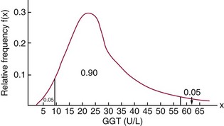
Frequency Distribution
Probability and Probability Distributions
Statistics: Descriptive Measures of the Sample

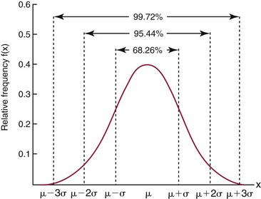
The Gaussian Probability Distribution

Student t Probability Distribution

Nonparametric Statistics
Basic Concepts in Relation to Analytical Methods
Calibration


Algebraic Form
Variables*
Parameters†
y = (a − d)/[1 + (x/c)b] + d
(x, y)
a, b, c, d
R = R0 + Kc/[1 + exp(−{a + b log[C]})]
(C, R)
R0, Kc, a, b
y = y0 + (y¥ − y0)(xd)/(b + xd)
(x, y)
y0, y¥, b, d
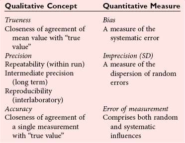
Trueness and Accuracy
Precision


Example


Precision Profile
Linearity
Analytical Measurement Range and Limits of Quantification
Analytical Sensitivity
 SDA at a 5% significance level. Historically, the meaning of the term analytical sensitivity has been the subject of much discussion.
Analytical Specificity and Interference
Analytical Goals
Qualitative Methods
Performance Measures
Agreement Between Qualitative Tests


Example

Method Comparison
Basic Error Model
Measured Value, Target Value, Modified Target Value, and True Value


![]()
Stay updated, free articles. Join our Telegram channel

Full access? Get Clinical Tree


Selection and Analytical Evaluation of Methods—With Statistical Techniques