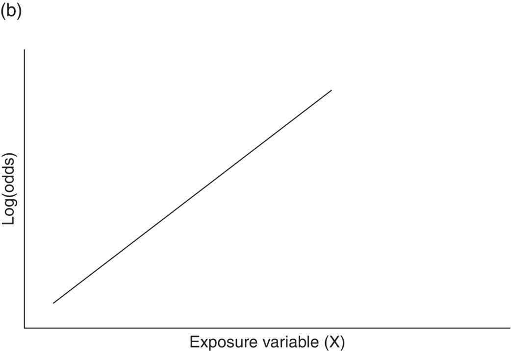
Chapter 4 The main limitation of most of the simple statistical methods in Section 3.4 is that they can only examine the relationship between one exposure and one outcome measure, each measured only once. In most observational studies, several factors are measured, or there could be several exposures of interest, and the aim is to examine these at the same time, including allowance for potential confounders. Regression analyses can do this easily, making them one of the most useful and common statistical methods for analysing observational studies. They come under the generic heading generalised linear models (the outcome measure, or some transformation of it, has a linear or straight line relationship with a set of factors) [1]. This chapter provides an overview of regression analyses. Regression analyses may appear complex, but although the calculations would not be performed by hand, they produce the same effect sizes covered in Chapter 3, with 95% CIs and p-values, which are interpreted in the same way. There are other analytical methods, some more complex, and occasionally, it may be necessary to develop one for a particular study design and analysis, because of limitations of other methods, with 95% CIs and p-values, which are interpreted in the same way. The following example highlights the general concepts underlying regression, using the simplest type, linear regression (or general linear model). In a study in which blood pressure (outcome measure) and age (exposure) are determined on 30 men, aged 40–70, in England (see the scatter plot Figure 4.1), two questions are of interest: Figure 4.1 Scatter plot of 30 measurements of age and blood pressure. If there were no association at all between blood pressure and age, the observations would generally lie horizontally. However, Figure 4.1 shows a clear tendency for blood pressure to increase with increasing age, and it appears that a straight line could be drawn through the observations. There are mathematical techniques for finding the straight line that, on average, is closest to all the points: called the linear regression line. The general form of a linear regression line is The regression analysis produces values for ‘a’ and ‘b’ (called coefficients): In the example, the form of the line is As with all summary measures, this line cannot perfectly represent all observations, that is, while some lie on or close to the line, others are far from it, such as the individual aged 54. The equation can also be used to estimate the average level of blood pressure for any given age: But this should only apply to men aged 40–70, for whom there were data in the analysis. Although a straight line fits the data in this age range well, the association could be quite different outside this range. A linear regression model assumes that the observations are independent, and the following are each approximately Normally distributed: (i) the outcome measure (y-variable) at any value of the exposure (x-variable), and (ii) the residuals (observed value minus the value expected from the regression line). Sometimes, the outcome measure and exposure are each checked to determine whether they are Normally distributed (see page 30), and if either are clearly skewed, a transformation of the data is used before fitting the regression line. The regression line comes from a sample of observations (30 men in the example), but the aim is to make inferences about the whole population of interest, that is, all men aged 40–70 in England. As with any other summary statistic or effect size, the regression coefficient (slope) will have an associated standard error, used to calculate a 95% CI: The standard error for the slope in Figure 4.1 is 0.162, so the 95% CI is 1.4–2.0 (Box 4.1). In the example, the p-value for the regression coefficient is < 0.001. This means that if it is assumed that there really were no association (i.e. the true slope is zero, the no effect value), a slope as large as 1.7 or greater could be found by chance alone in < 1 in 1000 similar studies of the same size. Therefore, the observed slope is unlikely to be due to chance, and so is likely to represent a real association between blood pressure and age. The p-value also allows for the possibility of the slope being −1.7 or lower (blood pressure decreases with increasing age), so it is a two-tailed p-value (as in Section 3.3), which is the most conservative and the one to interpret in most situations. Many observational studies are based on a large enough number of participants so that a few overly large or small data values should not greatly influence the results. Nevertheless, it is always worth checking the scatter plots for outliers. Figure 4.2a shows hypothetical data on blood pressure and age from 10 men, where there is no association (the slope is close to zero, 0.01). In Figure 4.2b, however, the presence of a single outlier creates a statistically significant negative association with slope −1.3. The line is trying to fit through all the data points, including the outlier, as best as it can, but as a result, it does not fit most of the observations. If data values like these are observed, they should be checked first to determine whether they are real or errors. If the value(s) is real, the regression analyses should be performed both with and without them, and the implications of both analyses should be discussed. Figure 4.2 Illustration of how a single outlier can create an association, when the other observations do not show any association. The 10 observations in (a) are the same as in (b). The type of outcome measure determines which effect size should be used, as well as the type of regression method (Box 4.2). These regressions all involve the same principle of trying to fit a straight line through something. This represents the simplest association to find and describe. Linear regression involves fitting a line through a continuous (outcome) measurement, while logistic, Cox, and Poisson regressions do this through some measure of risk. Risk can only take values between 0 (e.g. does not have a disorder) or 1 (does have the disorder), so the shape of risk in relation to an exposure variable would look like Figure 4.3a; it can rarely be a straight line. This can be overcome by a transformation, using risk expressed as an odds (see page 51). A logistic regression analysis uses logarithm of the odds, loge[risk/(1 − risk)], and the effect size it produces is an odds ratio (see page 51–52). With no upper or lower constraints, a straight line can be fitted, as with linear regression (Figure 4.3b). For time-to-event outcomes, the principle is similar to logistic regression, but loge of the hazard rate is used, and this is analysed using a Cox regression, producing a hazard ratio. The interpretation of 95% CIs and p-values are as before. Figure 4.3 Illustration of how a straight line cannot be fitted through risk (a), but it can through the logarithm of the odds (b). Each of the regressions in Box 4.2 produces an effect size. In the simplest case (one exposure and one outcome measure, each measured only once), they would be the same as those calculated by hand, for example: The simple logistic regression analyses presented earlier are based on a two-level outcome measure (e.g. dead or alive, developed disorder or did not, quit smoking or not). However, there are outcome measures with ≥3 levels, such as disease severity (none, mild, moderate, or severe). An easy approach is to collapse these into two levels, but information is then lost. Instead, an extension of logistic regression, ordinal logistic regression could be used. This produces odds ratios as before, but their interpretation is slightly different. Suppose the odds ratios in Table 4.1 came from an ordinal logistic regression where the outcome measure was severity of asthma among asthma patients: mild, moderate, or severe. Table 4.1 Hypothetical results from an ordinal logistic regression, where the outcome measure has three levels (mild, moderate or severe asthma). *Not on log scale. Suppose the exposure factor involves ‘taking measurements on people’ (continuous data), age: As age increases by 1 year, the odds of being in a higher asthma severity group increases by 1.37 (37% increase) compared with all the lower severity groups. That is: If the exposure factor involves ‘counting people’ (categorical data), for example, sex: The odds of being in a higher asthma severity group decreases by 0.75-fold compared with all the lower severity groups among females compared with males. That is: A key assumption with this method is that the effect is the same across all categories of the outcome measure; otherwise, the same odds ratio cannot be used to compare higher categories with all lower ones (as in the descriptions given earlier). A test of parallel lines can be produced by the regression analysis to assess whether this assumption is correct. Also, if the outcome measure has many levels, a linear regression model might be more appropriate. If the outcome measure has at least three levels, but there is no natural ordering to them, a multinomial (polychotomous) logistic regression could be used. One of the levels must be selected as the reference group, and an odds ratio is produced, which is the effect of each of the other levels, in comparison with the reference level. The interpretation of odds ratio is therefore not as simple as for logistic regression with a two-level outcome measure. Poisson regressions can be used for outcome measures that involve counts, including measuring risk of a disorder or death, for example: The effect size is the relative rate, which has a similar interpretation to relative risk. Examples are shown in Box 4.3. Poisson regression can allow for different lengths of follow-up (exposure time) for participants.
Regression analyses
4.1 Linear regression
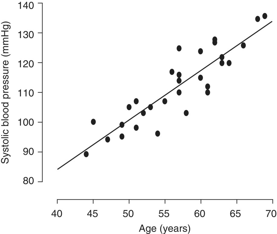


What could the true effect be, given that the study was conducted on a sample of people?

Could the observed result be a chance finding in this particular study?
4.2 Identifying and dealing with outliers
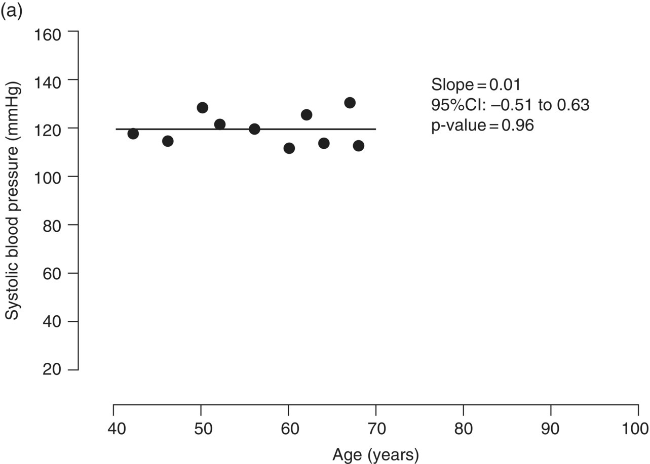
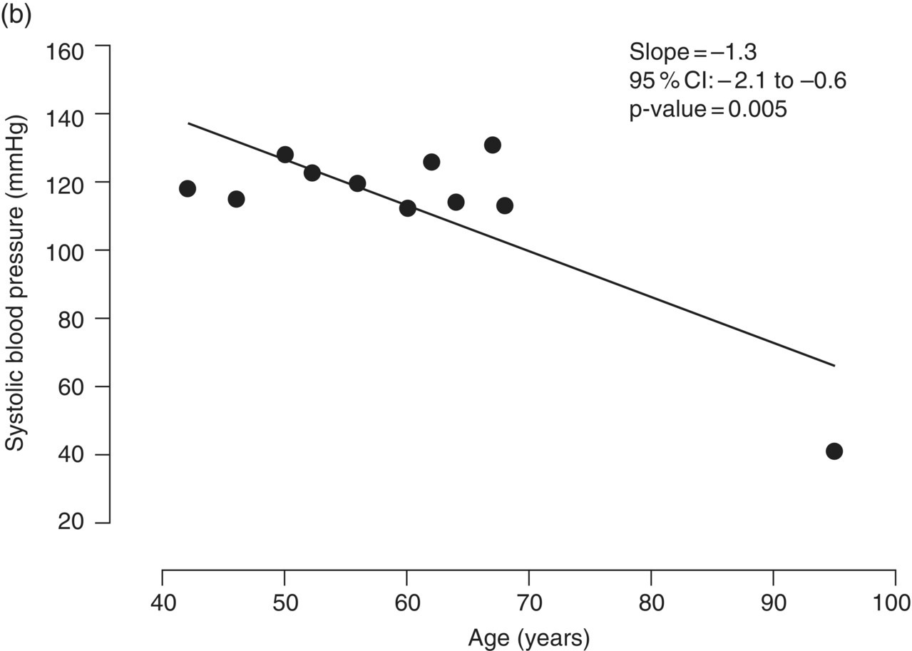
4.3 Different types of regressions
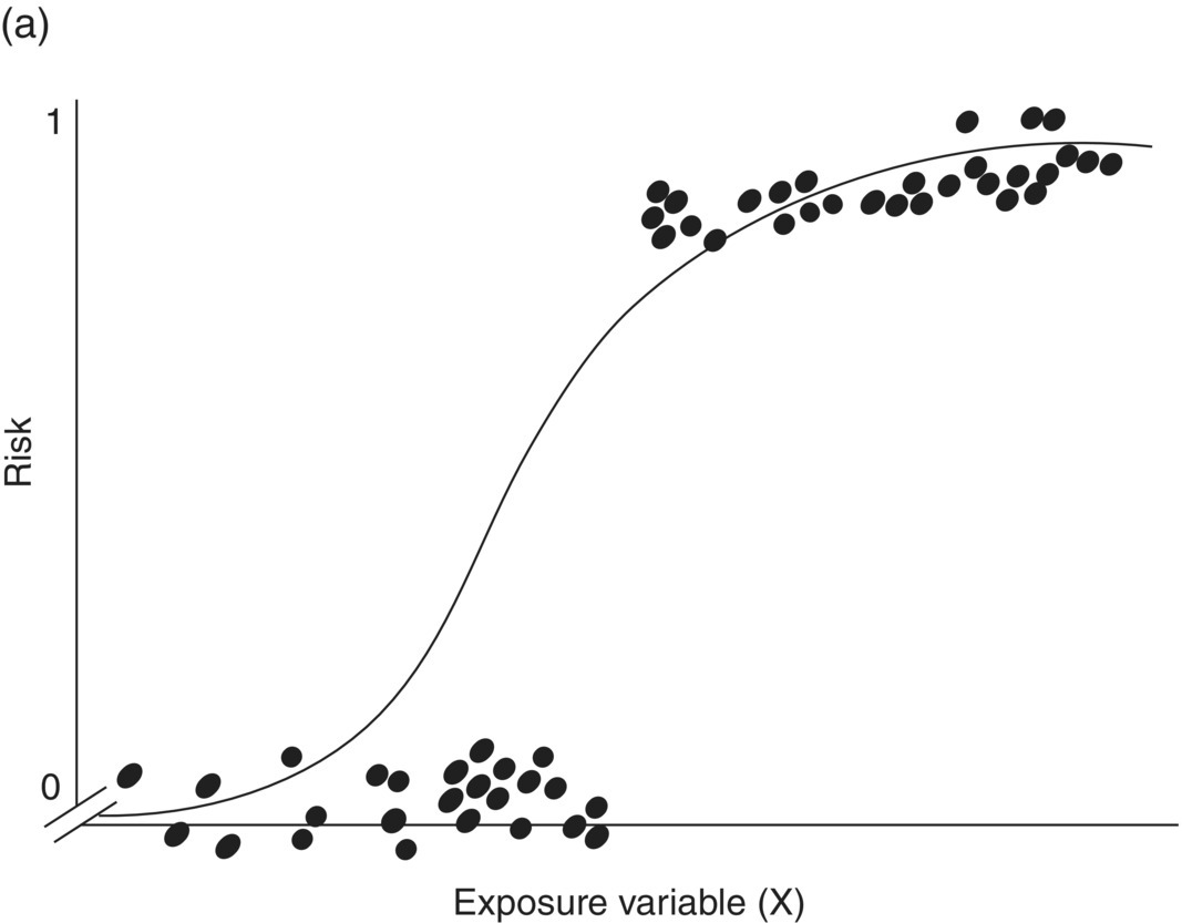
Ordinal logistic regression
Regression coefficient (odds ratio)*
Age (years)
1 year increase
1.37
Sex
Males
1.0
Females
0.75
Poisson regression
Stay updated, free articles. Join our Telegram channel

Full access? Get Clinical Tree


