The no effect value

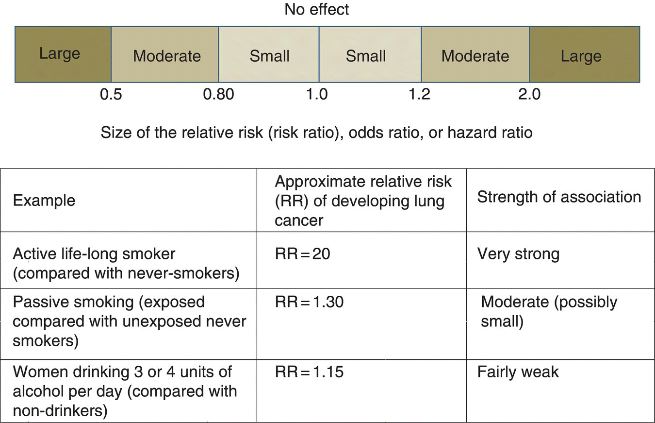
If there were no difference in alcohol drinking habits between the two groups, each would have the same risk of hazardous consumption. The relative risk (the ratio of the two risks) would be one, and the risk difference would be zero. These are called the no effect values, and they are used when interpreting confidence intervals and p-values (Sections 3.2 and 3.3).

Direction of the effect

Relative risk and absolute risk difference indicate the magnitude of the effect, but not the direction, that is, whether the outcome in one group is better or worse than another. This will depend on what is being measured (Box 3.3).

Converting relative risk to percentage change in risk

Relative risks of 0.5 or 2.0 are easy to interpret; the risk is half or twice as large as in the reference group. However, values of 0.85 or 1.30 are less intuitive; the risks are 0.85 or 1.30 times as large as that in the reference group. Converting relative risk to a percentage change in risk is an attempt to make it more interpretable (Box 3.4).

Relative effects (relative risk) or absolute effects (risk difference)?

Relative risk (risk ratio) and risk difference each provide different information about the study results. Relative risks tend to be similar across different populations, indicating the effect of an exposure generally. They do not usually depend on the underlying rate of disease. A relative risk of 0.5 means that the risk is halved from whatever it is in a particular population, for example, a background incidence of 1 per 1000 reducing to 0.5 per 1000, or 20 per 1000 reducing to 10 per 1000. However, risk difference reflects (depends on) the underlying rate, and so will vary between populations. It indicates the effect in a particular population, that is, a measure of impact.

As a disorder becomes more common, relative risk is not expected to change much, but risk difference will increase. An exposure has a greater impact on a population when the disorder is common. Table 3.1 illustrates this. Smoking is the strongest risk factor for those with the largest relative risks that is, lung cancer (14.6) and chronic obstructive pulmonary disease (COPD) (14.2), while there is only a moderate association between smoking and ischaemic heart disease (relative risk 1.62). However, the number of extra deaths among 100,000 smokers is 232 and 145 for lung and COPD, respectively, both of which are lower than the number of extra deaths due to heart disease, 382. Even though the relationship (relative risk) between smoking and heart disease is much weaker than for lung cancer, the impact on public health is greater, because heart disease is more common. Similarly, although there is a strong association for head and neck cancer (relative risk 6.7), there are only 51 extra cases per 100,000 smokers.

Because risk difference varies between populations, relative risk is the most commonly reported effect size. Risk difference should be examined in addition to relative risk when evaluating the impact on a population.

Relative risk or odds ratio?

An odds ratio is sometimes reported instead of relative risk. It has useful mathematical properties used by many statistical methods, especially the regression methods (Chapter 4). Risk and odds are different ways of presenting the likelihood of having a disorder (or other event):

Risk: 1/n, e.g. 1/10

Odds: 1/n–1, e.g. 1/9

The denominator for risk is all individuals, but for odds it is only unaffected individuals.

Table 3.2 illustrates odds ratio and relative risk, for different prevalence. In Table 3.2B, it would be incorrect to interpret the odds ratio of 14.8 as a 14-fold increase in risk (or 138% excess risk). The risk has been increased 2.5 fold (or 150%), indicated by the relative risk, but the odds in males are 14.8 times greater than the odds in females.

Odds ratio is the effect size calculated from case–control studies; cohort studies can be used to produce either an odds ratio or relative risk.

How big is the effect?

When interpreting relative risks or odds ratios, it is useful to judge whether the effect is small, moderate, or large. Although this can be a subjective exercise, it considers the importance of the association between an exposure and outcome measure in context. Figure 3.1 is an approximate classification.

Using relative effects can make the association between an exposure and outcome appear more important than it really is. An extreme example is shown in Table 3.3. The relative risk is 3 in both cases, representing a trebling of risk (or a 200% increase in risk) which is considered large, but the absolute risk difference in the second row of the table actually represents only two additional persons with the disorder among every one million exposed. This is a negligible effect, in terms of impact on a population. The classification of effects as small to large should therefore be applied separately to relative risk or absolute risk difference, and it may not be the same.

Risk of an event		Relative risk	Risk difference
Exposed	Unexposed
3 per 100	1 per 100	3	2 per 100
3 per 1,000,000	1 per 1,000,000	3	2 per 1,000,000

The effect size should be examined after adjusting for the effects of potential confounders (using regression methods in Chapter 4) otherwise conclusions on the relationship, especially if causality is inferred, could be questionable. Very large effects (e.g. a relative risk of 10 or more) are unlikely to be completely explained by confounding and bias, so if important confounding and bias have been ignored the conclusion probably remains the same, but there might be uncertainty over the size of the effect (the relative risk could be 5 instead of 10 after allowance for confounders, but 5 is still large). Small effects (e.g. relative risk 1.10) could be due to confounding or bias, so more care is needed when interpreting these.

Attributable fraction (or risk)

The risk in the exposed and unexposed groups can be used to calculate an attributable fraction, of which there are two forms (Box 3.5). Both assume that there is no significant bias or confounding; if there were, the estimates are likely to be lower. Attributable fractions can be used in addition to effect sizes when describing the impact of an exposure (risk factor) on a disorder in a population.