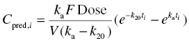
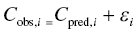
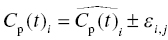
Many of the equations used to describe pharmacometric models have adopted letters of the Greek alphabet to represent particular model structures. Some of the more common Greek letters used are listed in Table 2.1.

2.2 Model Elements

A pharmacometric model is a mathematical-statistical construction that defines the relationship between dependent (e.g., concentration) and independent (e.g., time and dose) variables. The function of the model is to describe a system, as observed in a set of data. Models have several required elements: (i) a mathematical-statistical functional form (e.g., a compartmental PK model), (ii) parameters of the model, and (iii) independent variables that improve the ability of the model to describe the data. These three elements are given in the following example:

The dependent variable, concentration, is related to the prediction of a mathematical function implied by f(…), having parameters, θ, Ω, ∑, and independent variable elements of weight, dose, and time. When we fit a particular model to a collection of data, it is the parameters of the model that we are attempting to estimate.

There are two types of pharmacometric model parameters: fixed-effect and random-effect parameters. These are elements in the mathematical-statistical model. Parameters of both types take on a single numerical value in the model, but they represent different types of effects or elements in the model. Fixed-effect parameters are structural parameters that take on a single value that represents the population typical value of the parameter. Random-effect parameters also take on a single value for the population, but this value represents the variance of a distribution of some element of the model. Modeling a parametric distribution requires specification of, or assumptions about, three components of the distribution: (i) the shape of the distribution, (ii) the central tendency (e.g., the median or mean), and (iii) how much the individual values of the distribution vary around the central tendency (i.e., variance). Most applications of NONMEM (Beal et al. 2011) assume that the distribution of random effect terms represented in the model is symmetric, with a central tendency of zero. Parameter distributions that are not symmetric may be modeled through various transformations in the construction of the variance model. Here the underlying elements of the distribution being estimated are symmetric, but a transformation is used to model a distribution that is not symmetric. A common example is the use of a log-linear transformation. More complex transformations may be accomplished through logit, Box–Cox, heavy tailed, or other methods (Petersson et al. 2009).

The first two components of parametric distributions are satisfied by these assumptions and are generally not specifically stated with the model. The adherence of a model to these two assumptions can be tested in the model building process and evaluated from the NONMEM output. The third component is satisfied by estimating the population variance as a random variable.

2.3 Individual Subject Models

Traditional PK models for individual subject data define a set of fixed-effect parameters and mathematical structure that relate predicted concentrations to the observed data from an individual and include one level of random effect to account for the variance of the differences between observations and the model predictions (i.e., residual error). These models have a structural part, the PK model, and a statistical part, the variance model for the error between predictions and observations.

For example, the structural model for a one-compartment model with first-order oral absorption, illustrated in Figure 2.1, may be defined as follows:

where, k_a is the first-order absorption rate constant, V is the volume of distribution, k₂₀ is the first-order elimination rate constant, and F is the fraction of the administered dose that is available for systemic absorption. C_pred,i is the model-predicted concentration at the ith timepoint after the administration of a single dose.

In order to fit the model to a set of observed data, a statistical component of the model is needed to address the difference between the predicted and the observed concentrations.

For example, the aforementioned model might be fit to the observed serial concentration data from an individual following a single dose according to the following equation:

where, C_obs,i is the ith observed concentration in the individual, C_pred,i is the ith predicted concentration as defined earlier, and ε_i is the difference between the predicted and observed ith concentrations at time t_i. Through the model fitting process, point estimates of parameters are obtained for the structural model components: V/F, k_a, and k₂₀. These estimates define the structural PK model. One additional parameter (Ω for individual models or ∑ for population models) is estimated that describes the magnitude of the variance of the ε_i values across the observations of the individual. This parameter represents the statistical component of the model. A variety of statistical error models may be used, each with different assumptions about the nature of the differences between the observed and predicted data. These model components will be discussed more fully in later sections of this chapter.

2.4 Population Models

Population approaches in pharmacometric modeling extend traditional individual subject models by adding models that account for the magnitude, and sometimes the sources, of variability in model parameters between individuals. Population models typically include all the model components described earlier but also add parameters and submodels for the variations in structural model parameters between individuals or for variations in those parameters from one occasion to another within an individual. In population models, this leads to nested levels of random effects. The first level is at the parameter level and typically addresses the difference in the model parameters between subjects. The second level is nested within the first. In other words, there may be multiple observations at level two for each instance of the level-one effect. This second level is at the concentration level for PK models. These concepts will be discussed in further detail later in this chapter. The nesting of random effects to account for parameter differences between individuals is the greatest difference between individual and population models.

2.4.1 Fixed-Effect Parameters

Fixed-effect parameters are model elements that take on a particular, or scalar, value. They represent structural elements such as clearance or volume in a PK model. Within NONMEM, the standard nomenclature for a fixed-effect parameter is THETA(n), where n is an integer-valued index variable defining the particular element of the vector of all THETAs in the model. No value of n may be skipped in the definition of model parameters. For instance, there cannot be a THETA(2) in the model without a THETA(1). Writing the control files will be described in detail in Chapter 3, but note here that most code in the control file must generally be written in all uppercase letters. More recent versions of NONMEM allow some exceptions to this, but in this text, we will specify literal NONMEM code using all uppercase letters.

Individual subject models include fixed-effect parameters to describe the structural model (e.g., V_d/F, k_a, and k₂₀ in the aforementioned example) for an individual subject’s data. For instance, if we define the first-order absorption rate constant, k_a, as the first element of THETA(n), then

KA = THETA(1)

Here, THETA(1) is the element of the THETA vector used to estimate the typical value of the model parameter, k_a. The index value of THETA, n, is associated with a particular model parameter (e.g., k_a) through the code written in the control file. THETA(1) in one model might be used to model k_a, while in another model, THETA(1) might be used to model clearance.

With population models, fixed-effect parameters of the structural model define the typical values, or central tendencies, of the structural model parameters for the population. Thus, THETA(1) is an estimate of the typical value, or central tendency, of a parameter (e.g., k_a) in the population.

Fixed-effect parameters may also play a role as components of the variance model for a parameter, defining systematic, quantifiable differences in the parameter between individuals. For example, a possible submodel to describe the volume of distribution (V) might be the following:

V = THETA(2) + THETA(3)*WTKG

Here, THETA(2) defines the typical value of the portion of V that is not related to body weight. THETA(3) defines the typical value of the proportionality constant for that part of the volume that is proportional to body weight expressed in kilograms (WTKG). If this model is appropriate for a set of data, then THETA(3) explains at least some of the systematic difference in V between individuals.

Fixed effects may also be used as components of the residual variability (RV) model or for other modeling techniques. No matter how it is employed in a model, a fixed-effect parameter takes on a single, fixed value. This value is updated during the estimation process until convergence is obtained. The final fixed-effect parameter values of the model are those that minimize the objective function or meet other stopping criteria of the estimation method.

2.4.2 Random-Effect Parameters

For population models, random-effect parameters are components of the model that quantify the magnitude of unexplained variability in parameters (Level 1, L1) or error in model predictions (Level 2, L2). In other words, in population models, the L1 parameters quantify the magnitude of the differences of individual parameters from the typical value (i.e., parameter-level random error), and L2 parameters quantify the magnitude of differences between observed dependent variable values and their predicted values from the model (i.e., observation-level random error). For individual subject models, there is only one level of random effect, L1, which describes the observation-level random error. For the remainder of this section, models will be assumed to be population models with two levels of random effects.

Random-effect parameters describe the variance of a parameter, with an assumed mean of zero, as illustrated in Figure 2.2. The distribution of a random variable describing the difference between subjects in a parameter (e.g., eta-clearance) is typically assumed to be symmetric but is not required to be normal.

2.4.2.1 L1 Random Effects

For population models, L1 random effects may describe the magnitude of the differences in the values of parameters between subjects (i.e., interindividual variation) or the differences between occasions within a subject (i.e., interoccasion variability).

The vector containing the individual subject estimates of the L1 random-effect parameters is termed the ETA vector (i.e., η_i,n). In principle, η_i,n, is a vector of all the ETAs in the model for an individual, i, with n being an index variable to define the elements of the vector. Each subject will have her own η_i,n vector. The L1 random-effect parameter that is estimated is the variance of the distribution of η_i,n values. The standard deviation of the η_i,n values is ω_n. The variance is the standard deviation squared, . With NONMEM, the variance parameters are output in the omega matrix (Ω). If a population model is constructed with the following fixed and L1 random effects,

KA  = THETA(1)*EXP(ETA(1))

K20 = THETA(2)*EXP(ETA(2))

V  = THETA(3)*EXP(ETA(3))

then individual subject 1 will have one vector of estimates for η_1,1, η_1,2, and η_1,3. Other subjects in the dataset will have their own unique combination of values of these random effects. Taken together, all of the η_i,1 variables will have a variance that is reported in the omega matrix (Ω) in the diagonal element row = 1, column = 1 . The η_i,2 variables will have a variance that is reported as the (2, 2) element , and so on. The omega matrix for this simple example (shown here in lower triangular form) would be given as follows:

Ω =	0
	0	0

where, is the variance of the distribution of η_i,1 values across all subjects and thus describes the variance of k_a for this example. In the more general case, when covariance is estimated between random variables, the values can be understood as:

	Variance of ka
Ω =	Covariance of ka and k20	Variance of k20
	Covariance of ka and V	Covariance of k20 and V	Variance of V

Off-diagonal terms (row i, column j) represent the covariance between two parameters, i and j. Thus, is the covariance between k_a and k₂₀.

The off-diagonal terms are assumed to be zero unless they are explicitly modeled. To obtain individual subject estimates of the η_n,i values, a conditional estimation or post hoc Bayesian method must be used, and the individual subject values must be output in a table file in order to be accessible.

2.4.2.2 L2 Random Effects

L2 random effects describe the magnitude of unexplained differences between the predicted and observed values of the dependent variable. Considering the dependent variable to be plasma concentration, C_p, at time, t, in the ith individual

< div class='tao-gold-member'>

Only gold members can continue reading. Log In or Register to continue