Chapter 6 The appropriate interpretation of the output from NONMEM may well be considered the art in what is often referred to as the art and science of population modeling. The ability to understand the information provided in the various output files and to make appropriate decisions based on this information is one of the more challenging aspects of population modeling. With enough time and experience comes a knack for zeroing in on the most relevant bits of information from among the plethora of data provided in the output files in order to make appropriate decisions about what steps to take next. Although each modeling exercise is somewhat unique in its particular goals and objectives, the NONMEM output files contain a vast amount of information addressing various aspects of each model. Synthesizing this information to gain a complete and accurate picture of what can be learned from this particular model fit is essential to taking a logical path to a final model. The output described in this chapter will specifically focus on that of the classical estimation methods in NONMEM, though many of the comments are relevant to all of the estimation methods. After running a given typical model with NM-TRAN and NONMEM, several different files are available to the user. These include the *.rpt file, the *.FDATA file, the *.PRDERR file (possibly), the *.FCON file, and any user-requested files, such as the output from the $TABLE step(s) and/or a model specification file, and, with NONMEM version 7, the *.phi file, the *.ext file, the *.coi file, the *.cor file, and the *.cov file (Beal et al. 1989–2011). While each of these files contains important data and diagnostic information about a particular run, this chapter will focus primarily on reviewing the contents of the NONMEM report file. This file is the primary repository of results for a given model. Many of the additional files, now produced with version 7, such as the *.phi and the *.ext files, can be very useful to the user interested in programmatically parsing these output files for certain pieces of data to use as an input into another helper program or application. The NONMEM report file is a text file consisting of output from the various components of the NONMEM system relevant to a particular model fitting, in addition to error messages and other useful diagnostic data. In Sections 6.3.1–6.3.6 the specific types of output in the NONMEM report file will be reviewed in additional detail. The first section of output in the NONMEM report file consists of information relating to output from the NONMEM portion of the system. Recall that when the NONMEM program is used to run a particular population model, PREDPP may or may not be called, but NONMEM will be called. The output from each of these components of the NONMEM system is provided separately within the NONMEM report file. After the first few lines of output that detail the licensing information and version of NONMEM being called: the settings of various options are described, along with information regarding how NONMEM has read the data file with respect to the NONMEM-required data items:
Interpreting the NONMEM Output
6.1 Introduction
6.2 Description of the Output Files
6.3 The NONMEM Report File
6.3.1 NONMEM-Related Output
License Registered to: XXXX

Expiration Date: dd MMM yyyy

Current Date: dd MMM yyyy

Days until program expires : nn

1NONLINEAR MIXED EFFECTS MODEL PROGRAM (NONMEM) VERSION 7.X.Y

 ORIGINALLY DEVELOPED BY STUART BEAL, LEWIS SHEINER, AND ALISON BOECKMANN

 CURRENT DEVELOPERS ARE ROBERT BAUER, ICON DEVELOPMENT SOLUTIONS, AND ALISON BOECKMANN. IMPLEMENTATION, EFFICIENCY, AND STANDARDIZATION PERFORMED BY NOUS INFOSYSTEMS.
 PROBLEM NO.:1

 ‘text which follows $PROBLEM goes here’

0DATA CHECKOUT ….
0FORMAT FOR DATA: Among the items provided in this portion of the output, the total number of data records read from the dataset and the number of data items in the dataset are provided. Verification of these counts is an important step in ensuring that the data file has been read in correctly. The next portion of the output file provides additional counts which should be verified against checks of the data performed outside of NONMEM in order to ensure that the data have been read in correctly. The number of observation records and number of individuals in the dataset are provided (see the following): Since the observation record count is a tally of the records NONMEM considers as observation events (i.e., records where a PK sample or PD endpoint is measured), the difference between the number of data records in the dataset (provided earlier in the report file) and this count of observation records is usually the number of dosing records plus the number of other-type event records (i.e., where EVID = 2). The counts of the number of individuals and the number of observation records are perhaps most important to verify when the IGNORE and/or ACCEPT options are specified on the $DATA record. Since the specification of conditions within these options, especially multiple conditions, can be a bit tricky, the counts provided by NONMEM should always be confirmed with independent checks of the expected counts as a verification of the correct specification of the subsetting rules. Continuing with the NONMEM-related output in the report file, the next section of output reiterates the conditions (size and initial estimates provided) for the THETA vector and the OMEGA and SIGMA matrices. Next, the options requested for estimation and covariance via the $ESTIMATION and $COVARIANCE records are detailed in the output file. Finally, requests for specific output from the $TABLE and $SCAT records are described. The next section of the output file details the requests related to the call to PREDPP, if appropriate. When PREDPP is called (via the $SUBROUTINES record in the control stream), several PREDPP-required variables are needed in the dataset (and $INPUT record), and the coding of the model in the $PK block must correspond with the specification of the model requested through the choice of subroutines. If PREDPP is called, this section of the report file describes the model requested, the compartment attributes of that model and parameterization, the assignment of additional PK parameters, and the location of the PREDPP-required variables in the dataset. The next section of the report file is one of the most important sections for the analyst to review in great detail for each model before accepting or further attempting to interpret the results. For the first and last iteration and each interim iteration for which output is requested (via the PRINT = n option on the $ESTIMATION record), the following information is provided: the value of the objective function at this point in the search, the number of function evaluations used for this iteration, the cumulative number of function evaluations performed up to this point in the search. Also, for each parameter that is estimated, the parameter estimate is given in its original or raw units (with newer versions of NONMEM only), along with the transformed, scaled value of each parameter (called the unconstrained parameters (UCPs), which scale each parameter to an initial estimate of 0.1), and the gradient associated with each parameter at this point in the search (Beal et al. 1989–2011). The output from the monitoring of the search is provided as a summary of each step, with labeled information at the top of each section for the iteration number, the value of the objective function, and the number of function evaluations. Immediately following this information are specific lines of output for the parameters and the associated gradients for each iteration output. These columns are not labeled with respect to the corresponding parameter but are presented with the elements of the THETA vector first (in numerical sequence), followed by the elements of the OMEGA matrix and, finally, the elements of the SIGMA matrix. If a parameter was fixed (and not estimated) for a particular model, then a column would simply not exist for that parameter. So if THETA(4), the intercompartmental clearance term, was fixed to a value from the literature, the columns in the monitoring of the search section would be ordered as follows: THETA(1), THETA(2), THETA(3), THETA(5), ETA(1), ETA(2), etc., and then EPS(1), followed by any other EPS parameters which might have been used. In reviewing the detailed output regarding the search, it is important first to ensure that none of the gradients are equal to 0 at the start of the search. A gradient of 0 at the start of the search is an indication that there is a lack of information for NONMEM to use in order to determine the best estimate for that parameter. For example, this situation might arise if the model to be estimated includes an effect of gender on the drug’s clearance and the dataset consists entirely of males (the data in the gender column contains the same value for all subjects). In this situation, at the initiation of the search using the user-provided initial estimates, there would be no information to guide the search for an appropriate estimate of the gender effect, and the gradient would start at a value of exactly 0 for this parameter. In this case, no syntax errors would be detected, assuming the model was coded correctly and the variables needed to estimate the effect were found in the dataset. If a thorough EDA had been performed, the analyst would be aware of the gender distribution, and the attempt to fit such a model could have been avoided in the first place. However, assuming the situation may have arisen as an unintended consequence of data subsetting (perhaps via use of the IGNORE or ACCEPT options on the $DATA record), the gradients on the 0th iteration would be the first place to detect such a problem. One way to think about the value of the gradients is that the gradients provide information about the steepness of the slope of the surface with respect to a particular parameter at a specific point in the search. If you imagine the search process as a stepwise progression from some point on the inside of a bumpy bowl-like surface toward the bottom or lowest point of the bowl, each gradient describes what the surface looks like with respect to that parameter. If the gradient is high (a positive or negative value with a large positive exponent), then the surface is steep with respect to that parameter at that point and the search has not yet reached a sufficient minimum. If the gradient is small, either a value close to the final (best) estimate has been found or the model has settled into a local, not global, minimum with respect to that parameter. In addition to checking that the gradients generally get smaller as the search progresses and that no exact 0 values (or values very close to 0) are obtained, the gradients at the final iteration should be checked carefully as well. At the final iteration, all gradients should ideally have exponents equal to or less than +02, and of course, none should be exactly 0. Generally, the changes in the minimum objective function value from iteration to iteration will be greater at the start of the search than near the end of the search. When the search is nearly complete, the changes to the objective function value typically become very small. After the summary of the final iteration is provided, the happy phrase MINIMIZATION SUCCESSFUL may be found. This declaration is followed by a count of the total number of function evaluations used and the number of significant digits obtained in the final estimates. When the run fails to minimize for any reason, or minimizes successfully, but is qualified by some other type of warning or an indication of a problem(s) from the COV step, messages to this effect will be found in this general location in the report file. If an error occurs during the search, information about the error will be printed in the output file at the point in the search where it occurred. Overall, a great deal of information can be learned from a careful review of the output from the monitoring of the search. When errors do occur, the values of the gradients can provide clues about where the problems may lie. When the results are not optimal or do not make sense, the values of the gradients at the point at which the run completed its search may provide insight as to which parameters are causing the difficulty. When conditional estimation methods are used (e.g., FOCE, FOCE INTER, FOCE LAPLACIAN), additional information is provided following the summary of the monitoring of the search in the output file. Estimates of Bayesian shrinkage are provided for each of the estimated elements of OMEGA and SIGMA. Bayesian shrinkage is discussed in additional detail in Chapter 7. The mean of the distribution of individual eta estimates is also provided (referred to as ETABAR) along with the associated standard error for each estimate and the results of a statistical test of location under the null hypothesis that the mean of each element of OMEGA (i.e., each ETA) is equal to 0. If a p value less than 0.05 is reported, this is an indication that the mean of the distribution for that ETA is statistically significantly not equal to 0, or in other words, a rejection of the null hypothesis. Immediately following the monitoring of the search and related summary information about the run, the minimum value of the objective function is provided for the classical methods (FO, FOCE, FOCE with INTERACTION). After the minimum objective function value, the final parameter estimates are provided, first for the theta vector and then for the OMEGA and SIGMA matrices. Parameter estimates that were fixed in the control stream are reported in this section of the output as the fixed value without indication that the value of this parameter was fixed rather than estimated. Recall that in Chapter 3, a derivation was provided to calculate initial variance estimates for elements of OMEGA and SIGMA when an exponential or proportional error model is implemented, by working backward from an estimate of variability described as a %CV. This same derivation can be applied to the interpretation of the variance estimates obtained from NONMEM for elements of OMEGA and SIGMA. Typically, we wish to describe the magnitude of interindividual and residual variability in terms of a %CV, or at least a standard deviation (SD), which can then be compared in size to another estimate from the data. Let us begin with a diagonal OMEGA matrix, where each of the PK parameters upon which interindividual variability is estimated is modeled using an exponential error structure. So, a portion of our control stream code might look like the following: If the final parameter estimates obtained from NONMEM are the following:
(E6.0,E8.0, …
TOT. NO. OF OBS RECS: 1109

TOT. NO. OF INDIVIDUALS: 79
6.3.2 PREDPP-Related Output
6.3.3 Output from Monitoring of the Search
6.3.4 Minimum Value of the Objective Function and Final Parameter Estimates
6.3.4.1 Interpreting Omega Matrix Variance and Covariance Estimates
TVCL = THETA(1)

CL = TVCL*EXP(ETA(1))

TVV = THETA(2)

V = TVV*EXP(ETA(2))

TVKA = THETA(3)

KA = TVKA*(EXP(ETA(3))
OMEGA – COV MATRIX FOR RANDOM EFFECTS – ETAS *************
ETA1 ETA2 ETA3
ETA1
+ 3.62E-01
ETA2
+ 0.00E+00 1.19E-01
ETA3
+ 0.00E+00 0.00E+00 5.99E-01
we can calculate a corresponding approximate %CV for each variance estimate by taking the square root of the estimate and multiplying it by 100. So, in this case, the %CV of 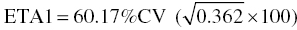 , of ETA2 = 34.50%CV, and of ETA3 = 77.40%CV.
If the error structures employed were additive instead of exponential or proportional (as may be used with PD parameters where the distribution may be normal as opposed to log normal), then we often describe the magnitude of interindividual variability in these parameters simply in terms of a standard deviation (SD). The SD can be obtained by simply taking the square root of the variance estimate. Assume that the following output was obtained regarding the magnitude of the ETA estimates for two parameters modeled with additive interindividual variability:
OMEGA – COV MATRIX FOR RANDOM EFFECTS – ETAS *************ETA1 ETA2
ETA1
+ 1.15E+01ETA2
+ 0.00E+00 2.03E+01
In this example, we can calculate a corresponding SD for each variance estimate by taking the square root of the estimate. So, in this case, the SD associated with 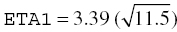 and with ETA2 = 4.51. Since these estimates are SDs, they maintain the same units as the parameter with which they are associated.
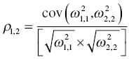
If a block structure was used to estimate off-diagonal elements of the OMEGA matrix (covariance terms), the interpretation of these estimates is also possible. To describe the magnitude of covariance between two random-effect parameters, a correlation coefficient can be easily calculated. Again, recall the information in Chapter 3 describing a method for obtaining an initial estimate for such a covariance term. We will use this method, working backward again, to derive a correlation coefficient from the covariance estimate.
If the following output is obtained in the report file,
OMEGA – COV MATRIX FOR RANDOM EFFECTS – ETAS *************ETA1 ETA2
ETA1
+ 3.61E-01ETA2
+ 2.01E-01 1.37E-01
we can use the following formula to calculate a correlation coefficient from these estimates to describe the relationship between the two variance estimates (Neter et al. 1985):