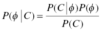
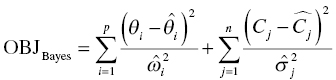
Bayesian methods in pharmacometric applications require the assumption of a prior population model structure and population parameter values, possibly including measures of uncertainty of the parameter values. With this information in hand, one may estimate the PK or PD model parameters for the individual. From the individual Bayesian model parameter estimates, one may then use the assumed model to reconstruct the concentration–time or effect profile for an individual and construct an estimate of the total exposure in the individual. This process is illustrated in Figure 7.1 and described later in this chapter.

A conceptual example of the power of this approach is illustrated here. Suppose one is exploring correlations between drug exposure and the occurrence of an adverse event (AE) to assess the safety profile of a drug product in clinical trials. If sparse concentration–time samples were collected from an individual in the trial and his dosing history is known, then Bayesian methods of individual parameter estimation can be used to reconstruct the concentration–time profile for the individual at any time in the trial. This is true even for cases of nonstationarity in PK such as enzyme induction or cases of nonlinearity such as capacity-limited absorption or metabolism, assuming the model adequately accounts for these processes. Using the individual PK parameter estimates, the dosing history, and the model, drug exposure on the day of an AE can easily be estimated. Estimated exposures at the time of the AE can be used along with estimated exposures in individuals not experiencing the AE to look for correlations between exposure and probability of occurrence of the AE.

Bayesian techniques are also useful in clinical practice settings. Much like traditional therapeutic drug monitoring (TDM) of certain drugs, population-based methods can be used to estimate PK parameters based on a single sample, a population model, and the patient’s dosing history. Where some traditional TDM approaches use simplifying assumptions or require sample collection to occur in a certain dosing interval or at a certain time within the dosing interval, population modeling methods with Bayesian parameter estimation may use data collected from an individual at any time during any dosing interval. Of course, collection of samples at some timepoints can be more informative to parameter estimation than others, but the availability of a model can even help in assessing this relative information content. Specialized software for TDM using population PK models and Bayesian techniques is available for clinical application. One such program is called BestDose® (Laboratory of Applied Pharmacokinetics, University of Southern California; (www.lapk.org)).

Individual PK parameter estimates also play an important role during model development for the purpose of identifying relationships between model parameter values and measurable covariates. This approach was previously described in Chapter 5.

This introductory chapter will not deal extensively with the theoretical aspects of Bayesian estimation, but after a brief introduction will focus instead on practical applications and methods used in drug development. The chapter presents methods for obtaining and using individual Bayesian or conditional parameter estimates when a population model is available using either the POSTHOC or the classical conditional estimation methods in NONMEM. The chapter does not focus on newer techniques available in the most recent versions of NONMEM that allow the specification of Bayesian priors when estimating the population parameters of a model, nor does it address $ESTIM BAYES method for parameter estimation.

7.2 Bayes Theorem and Individual Parameter Estimates

Bayes theorem was developed by Reverend Thomas Bayes and was published posthumously in 1763 (Bayes 1763). A review of Bayes theorem and its subsequent development and application in medicine was published on the 25th anniversary of Statistics in medicine (Ashby 2006).

In the context of PK, Bayes theorem can be considered as follows:

where ϕ represents the model parameter values and C represents the observed concentrations in the dataset. The probabilities in this equation are defined as:

• P(ϕ | C) is the conditional probability of ϕ given C or the posterior probability.
  
• P(C | ϕ) is the conditional probability of C given ϕ or the likelihood.
  
• P(ϕ) is the prior or marginal probability of ϕ.
  
• P(C) is the prior or marginal probability of C.

We are seeking the most likely set of parameters, given the observed concentrations in the individual [P(ϕ |C)]. These are technical statistical concepts and beyond the focus of this text. However, conceptual relationships important to Bayesian parameter estimation are illustrated in the following weighted least squares objective function, which can be considered to be a Bayesian objective function (Sheiner and Beal 1982; Bourne 2013):

where θ_i is the estimate of the individual’s parameter value; , , and are the fixed and random effects in the population model; and C_j and represent the observed and model-predicted concentrations.

Since the goal of the numerical estimation method is to minimize the objective function value, a few things can be noted about this Bayesian objective function. The first is that movement of an individual parameter away from the mean value (by increasing ) is discouraged unless there is a corresponding improvement in model fit to offset the increase in the objective function due to parameter value differences. If an individual has more observed data points, there is more opportunity to support moving a parameter away from the typical value in a direction that improves the fit of the model. When there are few or no data points that inform the estimation of a particular parameter, the value of that parameter will often shrink toward the typical value, since altering that parameter may have little influence on the values of individual predicted concentration values. The framework of this equation is also useful for illustrating the parsimony of this approach. Increasing the number of parameters without improving the fit of the model either increases the objective function or results in θ_i values that are essentially equal to so that .

Another observation related to this function is that when the variance of a parameter in the population ( ) is small, the change in the objective function with movement of the individual parameter from the typical value ( ) is magnified. Thus, if the underlying population variance in a parameter is small, a more substantial amount of improvement in the fit of the concentration data is required for each unit shift of the individual parameter away from the typical value. Conversely, if the variance of the parameter in the population is large, there is relatively less penalty in moving the individual parameter value away from the typical value.

A practical point is that one often finds that when there are too many parameters in a model so that the data are not informative regarding one or more parameters, the gradient estimation methods, such as FOCE, may wander, since they can change the parameter values without altering the objective function significantly. This can increase run times and lead to numerical problems in the estimation or covariance steps. We encounter this frequently when too many random-effect parameters are included and the data are insufficient to characterize them or when a model is overparameterized in fixed effects.

When we estimate individual subject parameters of the model (e.g., Cl_i), we are actually estimating the individual η values for the parameters that define the differences between the individual subject parameters from the typical population values of the parameters. For an individual then, we are drawing one instance of η from the distribution of η values defined with mean of zero and variance of ω². An example of individual PK model parameter definition is illustrated in the sample control code as follows:

  $PK

  TVCL = THETA(1)

  CL = TVCL * EXP(ETA(1))

The typical value of the parameter (TVCL) and the individual subject η-parameter value (ETA(1)) together define the value of CL (CL_i) for the individual subject. Also, note that Bayesian parameter estimates are only available for those parameters that include a defined η term. If only a typical value is included for a parameter in a model, then no individual-specific η may be obtained. Frequently, no η

Stay updated, free articles. Join our Telegram channel

Join