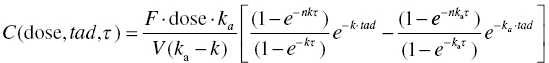
Chapter 10 Most of the discussion up to this point in our text has been in regard to pharmacokinetics (PK) alone. However, PK considerations in the development and clinical use of drugs generally have a supportive role. Primary questions of interest to the physician and pharmacist, once a particular drug has been selected for use, are how much and how often should the drug be administered to a particular patient. Though these are specifically kinetic concepts of extent and rate, the clinician is essentially asking questions of safety and efficacy, which when considered quantitatively we call pharmacodynamics (PD). PK questions are generally not primary, though they are an essential piece of the landscape over which the clinical decisions must be made. Definitions of acceptable safety and adequate efficacy are specific to each drug and indication. Defining these and determining the questions of primary interest during drug development require significant input from a multidisciplinary team including clinicians and thought leaders in the field. The team must understand the clinical context of the disease to be treated and of currently available drug therapy to effectively assess the potential for a new drug. Considerations of pharmacology, chemistry, pharmaceutics, regulatory, pharmacoeconomics, and other disciplines contribute valuable input to the team in constructing the questions of primary importance for the development of the product. Defining the primary questions to be addressed in the development program is often enabled by preparing a target product profile early in the development process. Crafting the target product profile encourages disciplined thought regarding the questions of interest and the data needed to address those questions. The pharmacometrician must translate these questions of interest into quantitative expressions and ensure that sufficient data are collected to allow the successful use of pharmacostatistical models to address these important questions. Perhaps of equal or greater importance to the value of their contribution, the pharmacometrician must be able to communicate the findings of modeling results to the team in clear terms that inform the decision-making process. Graphical representation of models and their implications can be of great benefit to that communication. A clinician does not need to understand the mathematical details of a complex system of differential equations in order to appreciate the behavior of a model and the extent to which this model answers interesting questions about drug effects. The pharmacometrician should compose the presentation of modeling results in a way that directly supports decision making by the project team. Pharmacometricians must have excellent modeling skills as well. Disease processes and drug action are complex in nature and require significant skill to model quantitatively. Frequently, PD models must consider issues of baseline response, relationship to PK, disease progression, development of tolerance, and many other factors. In addition, PD data may be continuous or discrete (e.g., binary or categorical). These considerations make PD models inherently more complex than most PK models. As an introduction to PK/PD modeling with NONMEM, this chapter will focus primarily on typical PD models of continuous data. The particular approach to implementation of PD models depends on the characteristics of the data and the questions to be answered. Direct linear or nonlinear regression can be performed between dependent and independent variables using $PRED. Alternatively, the PD model may be expressed using PREDPP in a couple of ways. If the PK model can be described by one of the specific ADVANs (i.e., ADVAN1–4 and 10–12), and the PD model is simple enough to be expressed algebraically, a specific ADVAN may be used with the PD model expressed in the $ERROR block. For more complex PK or PD models, the general ADVANs (i.e., ADVAN5–9 or ADVAN13) may be used. We will consider examples of each of these approaches in this chapter. In addition to considerations of which algorithms to use, there are a variety of modeling processes that may be followed in fitting PK and PD models. Since PK/PD models can be quite complex, the data and modeling process requirements must be considered carefully. PK/PD models can be developed by either simultaneously fitting the PK and PD parameters or by sequentially fitting the PK followed by the PD parameters. The selection of the process to use is at least in part, a balancing of the precision of the final parameter estimates against the substantial time requirements for execution of some processes. Simultaneous fitting of a PK/PD model is the most computationally intensive approach and typically the most time consuming. When a large number of parameters are being estimated simultaneously, models may suffer from stability problems in estimation, which will additionally prolong the run times. When the data are sufficient to estimate all the parameters simultaneously, this approach is considered the gold standard since there is interplay between the parameters of PK and PD in both directions (Wade and Karlsson 1999; Zhang et al. 2003). Sequential fitting is a two-step process. First, PK model parameters are estimated using a PK model and only the PK data. From these results, PK parameters or estimates of exposure are subsequently used as input in the PD model. This approach is easier to implement, and run times will generally be much shorter when compared to a simultaneous approach. Once the PK model has been estimated and parameters or exposure measures have been determined, there are at least three options for estimation of the PD model as shown in Table 10.1. First, the individual conditional estimates of parameters of the PK model can be fixed, while the PD model parameters are estimated using only the PD data. Second, the typical values of the population PK parameters can be fixed, while the PD model parameters are estimated using only the PD data. And finally, the typical values of the population PK parameters can be fixed, while the PD model parameters are estimated and have both the PK and PD data present in the dataset. Table 10.1 Three options for estimation of the PD models These PK/PD modeling approaches were described and compared by Zhang et al. (2003). These authors observed that sequential approaches minimize more quickly and more often, at least when using the classical estimation methods in NONMEM. In addition, when comparing the fitting options, sequential approaches that fixed the PK parameters to the population values, but included both the PK and PD data in the dataset were preferable, in that they yielded PD model parameter estimates that were similar in value and precision to those of simultaneous fitting, and did so in about 40% of the time required for simultaneous fitting. Using the $PRED block is efficient with relatively simple models such as some direct-effect models. Unlike PREDPP, PRED does not account for the context of the model; it does not have an internal representation of time or compartment amounts as PREDPP does. Thus, each record in the dataset must contain all of the information required for evaluation of the model, and no missing values are permitted, as these would be interpreted as zero values. Dataset construction for this type of model can be relatively simple since there are no dosing- or other-type records, and there is no continuity between records that must be built into the dataset, except that the records of an individual subject must be kept together. Other independent variables (e.g., treatment group, dose, concentration, exposure measure, sex, age, and weight) may be included in the dataset but must not be missing on any record if they are used in the model. These independent variables may be stationary or time varying. Sometimes, it is useful to include the subject’s baseline PD value as a separate (constant valued) data item. In this way, the baseline may be used as a covariate in the model, when appropriate, or it may be used for graphical or data summarization purposes. When using $PRED to implement a PD model, the control file must define the observed value of the dependent variable (Y) in terms of the individual predicted value (F), and a residual error term (EPS(i)). Pharmacokinetics may enter these models if the dataset contains the needed concentration values on each record, or if the concentration is predicted through algebraic equations using only the information available from each record. The latter is sometimes more complex in multiple-dosing situations since PRED does not account for the dosing history of a patient. The algebraic equations must themselves include the multiple dosing nature of the data. This is achievable for some circumstances, but will generally require the assumption of constant dose amounts given in equal and precise dosing intervals, since no dosing records are included in the dataset for a model specified through $PRED. An example of the utility of the PRED approach is the exploration of a relationship between maximum drug concentration (Cmax) and maximum change from baseline in corrected QT interval of the electrocardiogram (ΔQTc). This example is not put forward as an endorsement of this approach to the analysis of such cardiac data but is simply used as a demonstration of how one might code this type of model using $PRED. Each record in the dataset contains both a PK value (Cmax) and a PD value (ΔQTc). A few rows of data might be constructed as shown in Table 10.2. Table 10.2 Example of data for use with a model in $PRED With a single observation per subject, two levels of random effects would be confounded, and the model would not be identifiable. In this simple example, with one observation per subject, one might structure a linear model with a single level random effect (L1) as follows. The ID data item is dropped by NMTRAN, since with only one random-effect level all data are treated as if they come from a single subject, or more precisely, there is no subject level in the model. The PD value is the DV under analysis, and thus the DQTC data item is identified in the $INPUT line as the DV data item. The independent variable, CMAX, is an element of the dataset and defined in the $INPUT statement. The model relates these independent and DVs through a linear regression model. INT and SLP are the intercept and slope parameters of the linear model, respectively. EFF is the predicted effect, or ΔQTc. ΔQTc is identified as the DV data item, and thus is associated by NONMEM with the Y value in the residual error model. This association is made automatically by NONMEM. The residual error model, or the relationship between Y and the predicted value, EFF, is defined explicitly. Note that because IGNORE = C is included on the $DATA statement and the first character of the first row of the dataset is a C, this header row is dropped by NMTRAN when the data file is read. In this way, the header row can be included for the human reader of the dataset, but the character data are dropped as required when NONMEM reads the dataset. The following is another example of a direct-effect model coded using $PRED, which in this case uses a PK value from the dataset (CONC) to fit a Hill function with multiple random effects to a set of PD data. Estimating multiple levels of random effects assumes we have multiple observations per subject, at least for many members of the dataset. Here, CONC is the simultaneous drug concentration eliciting the immediate reduction in PD response. The ETA terms are level 1 random effects describing intersubject differences in PD parameters. EPS(1) is a level 2 random effect of the residual error model. Level 1 effects are constant for the individual and vary between subjects. Level 2 effects are at the observation level and differ between observations within a subject. No PK model is assumed or estimated in this example. PK is included simply as the concentration measurements obtained simultaneously with the PD measures. Using this approach, a PK value is required with each PD value. If the PK value were not present, either the corresponding PD value would have to be dropped, or a PK value would have to be imputed, perhaps through some interpolation or assumption of the model. In this example, the PD baseline value is estimated in the model. Even in cases where the baseline is measured, one might want to not only include the measured baseline value as the first record in the dataset for each subject but also estimate the baseline as a parameter of the model. If we use the observed baseline as a fixed value, then we assume we know the value without error. Modeling the baseline as a parameter allows us to estimate the magnitude of variability in the baseline and explore the influence covariates may have in explaining that between-subject variability. As mentioned previously, we may also want to keep the baseline value as a constant valued data item on every record (in a separate column from the DV column) in order to use the baseline as a covariate on other parameters in the model. Direct-effect PK/PD models can also be constructed where the PK concentrations are computed from individual subject parameters. For example, concentrations at any time-after-dose, tad, in the nth dosing interval of length, τ, for a drug having first-order absorption and first-order elimination can be predicted with the following equation:
PK/PD Models
10.1 Introduction
10.2 Implementation of PD Models in NONMEM
Option
Parameters that have fixed values
Dataset for estimating PD model contains
1
PK = Individual estimates
PD observations
2
PK = Population estimates
PD observations
3
PK = Population estimates
PK and PD observations
10.3 $PRED
10.3.1 Direct-Effect PK/PD Examples: PK Concentrations in the Dataset
CID
DQTC
C max
1001
3.6
54.9
1002
4.9
48.6
1003
2.1
35.2
1004
6.3
65.1
1005
5.2
55.6
1006
3.5
40.2
…
…
…
$PROB QTc, PRED
$INPUT ID=DROP DQTC=DV CMAX
$DATA data.csv IGNORE=C
; Since the header row
; starts with a C, that row
; is dropped
$PRED
INT = THETA(1)
; Intercept
SLP = THETA(2)
; Slope
EFF = SLP*CMAX + INT
; Drug effect model – linear
Y = EFF + ETA(1)
; Residual error model –
; additive
$EST PRINT=5 MAX=9999 SIG=3
$THETA
0.1
; Intercept
0.5
; Slope
$OMEGA
0.04
; Magnitude of Additive error
$PRED
EMAX = THETA(1) * EXP(ETA(1))
; Emax – maximum effect
EC50 = THETA(2) * EXP(ETA(2))
; EC50 – conc. of half
; Emax
GAMMA = THETA(3)
; Gamma – shape
; parameter
BL = THETA(4) * EXP(ETA(3))
; Baseline PD value
N = EMAX * (CONC**GAMMA)
; Numerator-Hill
; Equation
D = (EC50**GAMMA) + (CONC**GAMMA)
; Denominator-Hill
; Equation
EFF = BL – (N/D)
; Effect of drug is to
; decrease the baseline
Y = EFF + EPS(1)
; residual error model
10.3.2 Direct-Effect PK/PD Example: PK from Computed Concentrations
PK/PD Models
Only gold members can continue reading. Log In or Register to continue

Full access? Get Clinical Tree


