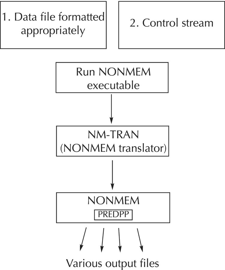
Chapter 3 After describing the main components of the NONMEM system, this chapter will provide a detailed explanation of the essential elements of coding an NM-TRAN control stream. Since NONMEM is run in batch mode (i.e., programs or control streams are written and submitted for execution all at once and not line-by-line), the coding of the NM-TRAN control stream is the fundamental building block upon which the rest of the system is built. Therefore, a solid understanding of how to code simple control streams is required before building up to more and more advanced and complicated examples. This chapter will describe many of the common control stream records, explain the various options that may be used with each, and provide examples of typical control stream statements. The NONMEM system consists of three major program components: NM-TRAN, the NonMem TRANslator; PREDPP, subroutines for the PREDiction of Population Pharmacokinetic models and parameters; and NONMEM, the engine for the estimation of NONlinear Mixed Effect Models. NONMEM, the heart of the program, consists of FORTRAN subroutines that govern the estimation of parameters of nonlinear mixed effects models. As such, NONMEM is by no means limited in its application to population and individual pharmacokinetic (PK) and pharmacokinetic/pharmacodynamic (PK/PD) applications. That being said, the PREDPP library of specific subroutines provides the pharmacometrician with access to multiple prewritten subroutines for many common and typical PK models, all of which can be customized to meet the individual needs of a particular compound to facilitate model development. The language we as modelers use is provided in NM-TRAN, the framework for the specification of the models, as well as the interaction with the system as a whole (Beal et al. 1989). While many interfaces and helper programs have been developed over the years to facilitate interactions with NONMEM, the NONMEM system itself can be thought of as a batch programming language. An NM-TRAN control stream is written and executed by the modeler. This control stream, in turn, calls the NONMEM dataset file (described in detail in Chapter 4) and the appropriate subroutines to complete execution of the specified model and return various files for review. There is no graphical user interface to open and no windows or drop-down boxes available from which to select model features or options. For this reason, the learning curve for proficiency with the use of NONMEM is a bit steeper than for many other programs that allow for a trial-and-error clicking approach. This text is intended to help ease that learning curve. Figure 3.1 graphically depicts the interactions of some of the main components of the NONMEM system. The NM-TRAN control stream, along with a separate data file, is created by the user. Typically, when the NONMEM executable is called, the user files are passed through NM-TRAN first, which parses each for syntax and formatting issues and then converts each file to a version appropriate for NONMEM. NM-TRAN also calls the appropriate FORTRAN subroutines, based on the specification of the model, and sends them to the FORTRAN compiler for compiling and loading. If PREDPP is also called (based on the control stream specifications), the generated PK and ERROR subroutines, along with the NONMEM-ready control file and data file, are then passed through NONMEM for estimation or other steps based on additional specifications in the control stream. Various NONMEM output files are generated, some by default and others optionally, again based on the specifications in the control stream (Beal et al. 1989). Figure 3.1 Schematic illustrating the components of the NONMEM system. The focus of the remainder of this chapter will be on the development of the NM-TRAN control stream, the program or instruction file, in which the model and various options for its estimation and requested output are specified. The reader is referred to User’s Guide IV: NM-TRAN or the online help files for additional information about each of the records and options described herein (Beal et al. 1989). The information provided in this chapter will aim to provide the novice user with the essential information needed to understand how to write a typical NM-TRAN control stream for the estimation of a simple PK model. The NM-TRAN control stream file is an ASCII text file, usually written with an available text editing tool, such as Microsoft WordPad®, Notepad, emacs, vi, or other NONMEM-friendly text-editing applications. Since the file must be saved as a plain ASCII text file, editing in a word processing program, such as Microsoft Word®, is possible, but not recommended, as the modeler must always remember to change the save settings in order to save to a plain (DOS) text file. The NM-TRAN control stream file is made up of a series of defined records and blocks of code, each of which starts with a particular string of characters following a dollar sign (“$”), which denotes the start of a new record or block of code to the program. For all record identifiers, a shorthand version of the record identifier name is available, consisting of at least the first three characters of the record or block name (e.g., $PROBLEM can be abbreviated to $PROB or even $PRO). Within the control stream file, blank spaces are allowed both between records and between options within a particular record. Although more recent versions of NONMEM now allow the use of tab characters in certain circumstances (where previously not allowed), it has been the author’s experience that it is safer to simply avoid the use of tabs in control streams (or data files). In the cases where syntax rules and options have changed over time with subsequent versions of NONMEM, it will be specifically noted. Each record in the control stream can be a maximum of 160 characters in length. For versions of NONMEM prior to 6.2, records of no more than 80 characters in length were allowed. Records that must extend beyond the allowable limit can continue after pressing the enter key. This rule also applies to the individual lines of code within a block statement, such as the $PK or $ERROR block. In these sections of code, equations must be broken up into parts, each less than the allowable line length and then combined together, as appropriate, in a separate equation(s). With NONMEM version 7.2 and higher, mixed case (a combination of upper and lower case) is permitted within the control stream. With versions prior to 7.2, however, all portions of the control stream, with the exception of file names, must be in all uppercase letters. Comments are permitted anywhere within the control stream, and are prefaced with a semicolon. Any text between a semicolon and the end of the line is considered a comment and not read by NM-TRAN. For early versions of NONMEM (prior to 7.0), a return was required after the last character in the control stream in order for the last record to be recognized. A control stream is provided in the following example for reference and to visualize the file elements to be discussed throughout this chapter. As described earlier, the statements in this example are not all-inclusive, nor are all the options specified in the records shown; this is merely an example of a typical PK model specification using NM-TRAN. Example NM-TRAN control stream for a simple one-compartment PK model
NONMEM Overview and Writing an NM-TRAN Control Stream
3.1 Introduction
3.2 Components of the NONMEM System
3.3 General Rules
$PROBLEM Example NM-TRAN Control Stream for a 1-cmt Model

$DATA /home/pathtomydatsaset/datafilename.dat IGNORE=#

$INPUT ID TIME AMT DV CMT EVID MDV

$SUBROUTINES ADVAN2 TRANS2

$PK
TVCL = THETA(1)
CL = TVCL * EXP(ETA(1))
TVV = THETA(2)
V = TVV * EXP(ETA(2))
TVKA = THETA(3)
KA = TVKA
; scale predictions based on dose (mg) and Cp (ng/mL)
S2 = V/1000
$ERROR
Y = F*(1 + EPS(1))
$THETA (0, 3.9) ; Clearance (L/h)
(0, 52.1) ; Volume (L)
(0, 0.987) ; Absorption Rate (1/h)
$OMEGA (0.09) ; IIV on CL (use 30%CV as init est)
(0.16) ; IIV on V (use 40%CV as init est)
$SIGMA (0.04) ; RV (use 20%CV as init est)
; Use conditional estimation with interaction
$EST METHOD=1 INTER MAXEVAL=9999 PRINT=5 MSFO=example.msf
$COVAR PRINT=E
Typically, the first record of an NM-TRAN control stream, the $PROBLEM record, is a required record that serves as an identifier for the control stream as a whole, allowing the user a space to label the file descriptively for later reference and identification purposes. The text that the user writes following the $PROBLEM record identifier is copied to the output file as a title, of sorts, for that file and to link together the problem specification and the results. If your practice is to modify or edit your most recent control stream to the specifications of the new model you wish to run (as opposed to starting with a blank page for each new control stream you write), it is good practice to train yourself to always start with modification of the $PROBLEM record to match your new purpose, before going on to the other required changes. A systematic method for describing models and naming files is helpful in maintaining some sense of organization as you add more and more complexity to your models. Another good practice involves adding a more complete header using commented text (i.e., following a semicolon “;”) to the top of each new control stream, to be filled in before saving and running the file; such a header might include the control stream author’s name, a date/time stamp, a section where the author can describe the purpose of the control stream, and the data file to be used. The $DATA record is used to indicate to NM-TRAN where to find the associated data file for the problem. The relative or complete filepath is provided, along with the data file name. Note that the appropriate specification of the filepath is based on operating system/environment-dependent syntax. The examples in this text use the forward slash “/” symbol to denote the separation between various subdirectories, as would be appropriate for a UNIX- or Linux-based system. Many Windows-based systems will use a backward slash “\” for this purpose and filepath specifications will begin with the drive (e.g., C:\My Documents\…). See the example control stream in Section 3.3 for a typical $DATA record specification. Additional options (i.e., IGNORE and ACCEPT) for subsetting the data for use with a particular model are also available with the $DATA record. The simplest method of subsetting the dataset requires modification to the data file itself, in conjunction with the use of a particular version of the IGNORE option of $DATA. To use this particular feature of the IGNORE option, a character is inserted in the left-most position of a particular dataset record intended for exclusion. The inserted character value (most ASCII characters are fine to use, except “;”) is placed on only those records selected for exclusion, and the records not selected for exclusion are left unchanged. Typically a “#,” “@,” or “C” is used for this purpose. If the “#” is used, NM-TRAN’s default behavior is to exclude those records containing this value in the first column and no extra option on $DATA is required. However, if a different character is used (e.g., “@”), the $DATA record would read: where “@” would be whatever character was used in the dataset to indicate such exclusions. In this case, as NM-TRAN reads in the datafile, all records with an “@” in the first column will be skipped over and not retained in the NONMEM version of the datafile used for processing and estimation of the model at hand. Such exclusions from the datafile can be confirmed by viewing the FDATA output file and also by checking the number of records, subjects, and observation records reported in the report file output (see Chapter 6 for additional information on where to find this information in the output file). If the exclusions to be tested are recognized at the time of dataset creation, the inclusion of an additional column or columns containing exclusion indicator flags may be considered. Suppose a variable called EXCL is created with values of 0, 1, and 2, where 0 indicates that the record should not be excluded, and 1 and 2 indicate different reasons for possible exclusion. To take advantage of this data field, another type of IGNORE option is available whereby the $DATA record may be written as follows: or or This type of conditional IGNORE option may be used in conjunction with the IGNORE=# type of exclusion described previously to exclude both records with a “#” in the first column in addition to those records that meet the criteria contained within the parentheses in the aforementioned examples. In this case, the IGNORE option would be included twice, perhaps as follows: While these options are clearly quite useful to the modeler, the real advantage lies in the fact that the dataset need not be altered to accomplish this latter type of subsetting, allowing different subsets of the data to be specified quite simply with different control stream statements. The conditional IGNORE option may be used with any variable or variables (i.e., data items) read in on $INPUT, including those not specifically created to deal with possible exclusions (in addition to those dropped with the “=DROP” option, see Section 3.4.3). In this way, the data file may be subset to include, for example, only those subjects from a particular study, only those subjects weighing more than a certain value, or even to exclude those subjects with a particular level of disease severity. Another important use of this feature is to temporarily exclude one or more observations in order to assess their influence on the model fit, as when a small number of concentrations are associated with high weighted residuals during model development. To use a single conditional argument, the syntax is as described earlier: NONMEM also allows more than one conditional argument to be used to express more complicated exclusion criteria with the IGNORE option; however, if more than one conditional argument is used, the conditions are assumed to be connected by an “.OR.” operator. No other operator may be specified with this option. Therefore, if one wishes to exclude those records where a subject’s weight is greater than or equal to 100 kg OR a subject is from Study 301 from the dataset for estimation, the $DATA record may be specified as follows: Note that the additional conditional statement is specified within the same set of parentheses, followed by a comma. In fact, up to 100 different conditional arguments may be specified in this same way with a single IGNORE option. The converse of the IGNORE option is also available—the ACCEPT option. ACCEPT may be specified with conditional arguments in the same way as IGNORE, also assuming an “.OR.” operator when multiple conditions are specified. Similar to IGNORE, the ACCEPT option may be used in conjunction with the IGNORE=“#” option, but may NOT be used in conjunction with an IGNORE option specifying conditional arguments. To illustrate the use of this option, if one wishes to include only those records where weight is less than 100 kg OR the study is not 301 in the dataset for estimation, while still excluding those records with a “#” in the first column, the $DATA record may be specified as follows: Now, there may be situations where the easiest and most intuitive way to envision the subsetting rules is with an “.AND.” operator. In those cases, consider the following helpful trick to coding an implied “.AND.” using the available implied “.OR.” If one wishes to exclude the subjects in Study 101 AND with disease severity greater than or equal to level 2 (i.e., exclude STDY.EQ.101.AND.DXSV.GE.2—a statement that would not be allowed by NONMEM in an IGNORE option due to the “.AND.”), as shown in Table 3.1 where the desired exclusion is indicated in black, this may be coded with the following $DATA record: Table 3.1 Desired inclusions and exclusions of data, based on study number and disease severity Another option some users may find helpful with $DATA is the CHECKOUT option. When this option is specified on the $DATA record, the CHECKOUT option indicates that the user desires to simply perform a check of the dataset based on the corresponding data file, $INPUT, and other records in the control stream. With this option, no tasks in the control stream other than $TABLE and $SCAT are performed (see Section 3.9). Furthermore, items requested in $SCAT should not include WRES which will not be computed with such a checkout run. Using the dataset only, table files and scatterplots will be produced, if requested, in order to allow the user to confirm the appropriateness of the dataset contents with regard to how it is read into NONMEM via $INPUT. The $INPUT record is used to indicate how to read the data file, by specifying what variables are to be found in the dataset and in what order. After $INPUT, the list of variables is specified, corresponding to each column of the dataset, using reserved names for variables where appropriate (see Chapter 4 for a complete description of the required variables for NONMEM and PREDPP). The list of variables to be read can include no more than 50 data items; with NONMEM versions 6 and earlier, only up to 20 data items were allowed in $INPUT. Since it is not uncommon to create a master dataset containing all of the relevant variables for modeling as well as many others that may be needed only to comply with regulatory submission standards, datasets may often contain more than the 50 (or 20) allowable fields. However, there is an $INPUT record feature that can be employed to accommodate this situation. If the data file includes more than the allowable maximum number of variables, certain variables not needed for the particular model estimation may be dropped by specifying their name in the list with an “=DROP” modifier after the variable name. So, if the dataset contains many demographic variables, only a small handful of which are to be used in a given model, the others in the list may be specified with the “=DROP” feature. Any conditional subsetting requested via the IGNORE or ACCEPT options of $DATA is performed prior to dropping variables via $INPUT, so even those variables intended to be dropped may be used to specify data subsets to NM-TRAN. In a similar way, if a name other than the reserved variable name is preferred for a particular variable (e.g., DOSE instead of the reserved term AMT), the nickname feature used to drop variables can also be used to assign an alternate variable name; in this case, the variable AMT would be specified as AMT = DOSE. Use of this feature ensures that the variable is read in correctly with the reserved name and that the alternate name is used in any output referring to this field. Furthermore, if characters such as “/” or “-” are used within a date format, the DATE variable must be read in with the “=DROP” modifier, although it will, in fact, not be dropped at all, but read by NM-TRAN and used in conjunction with the TIME variable to compute the relative time of events. The specific options for reading in date and time information are discussed in detail in Chapter 4. When PK models are to be specified, the library of specific subroutines available in PREDPP may be utilized. The $SUBROUTINES record in the NM-TRAN control stream identifies to PREDPP which subroutines to use based on the model structure and desired parameterization. A typical $SUBROUTINES record consists of the choice of a particular ADVAN and a particular TRANS subroutine, each identified by number. For example, the ADVAN1 subroutine contains the appropriate equations for a one-compartment model with first-order elimination, the ADVAN2 subroutine contains the appropriate equations for a one-compartment model with first-order absorption and elimination (thus allowing for oral or subcutaneous dosing), the ADVAN3 subroutine contains the appropriate equations for a two-compartment model with first-order elimination, the ADVAN4 subroutine contains the appropriate equations for a two-compartment model with first-order absorption and elimination, the ADVAN11 subroutine (numbered so because it was added to the PREDPP library years after the core set of ADVANs1–10 were developed) contains the appropriate equations for a three-compartment model with first-order elimination, and the ADVAN12 subroutine contains the appropriate equations for a three-compartment model with first-order absorption and elimination. While this chapter focuses on the specific ADVANs, the more general linear and nonlinear ADVANs are discussed in Chapter 9. Here, the reader is referred to User’s Guide VI: PREDPP or the online help files for more detailed and specific information about each of the available subroutines in the PREDPP library (Beal et al. 1989). While the specific ADVAN routines define the particular model to be employed, the corresponding TRANS subroutines indicate how the parameters of the models should be transformed, or in other words, which parameterization of the model is preferred. TRANS1 subroutines, which may be used with any of the specific ADVAN routines discussed earlier, parameterize the models in terms of rate constants for the first-order transfer of drug from compartment to compartment, or k10, k12, k13 types of parameters. TRANS2 subroutines, also available with any of the specific ADVAN subroutines described so far, parameterize the models in terms of clearance and volume terms. Alternative TRANS subroutines are available for select ADVANs, offering additional options for parameterizations in terms of clearance and volume parameters or exponents (i.e., α, β, γ, and so on). It is this combination of the selected ADVAN and TRANS subroutines on the $SUBROUTINES record that determines which required parameters must be defined, and which additional parameters are recognized and also available for estimation. Table 3.2 provides the required and additional parameters available for select ADVAN and TRANS combinations. For example, with the ADVAN2 and TRANS2 subroutines selected on the $SUBROUTINES record, the required parameters include CL, V, and KA. Additional parameters including F1, S2, ALAG1, and others are also available and may be assigned and estimated, if appropriate. If the ADVAN3 TRANS4 combination is specified in $SUBROUTINES, then CL, V2, Q, and V3 parameters would be the required parameters and a variety of additional optional parameters would be available as well. As described in Section 3.5.2, equations must then be written to define each of the required parameters and any additional parameters used. The reader is referred again to User’s Guide VI: PREDPP or the online help files for the relationships between the required parameters of each of the ADVAN and TRANS subroutines (Beal et al. 1989). Table 3.2 Required and additional parameters for select ADVAN and TRANS subroutine combinations With the appropriate subroutines called, the variables of the model are the next item to be specified in the control stream. This includes the assignment of thetas and etas to the required (and additional) parameters based upon the selected ADVAN and TRANS subroutine combination, and the random-effect terms for interindividual variability in PK parameters. These are specified and assigned within the $PK block. The $PK block (and other block statements to be discussed subsequently) differs from the NM-TRAN records described thus far in that following the block identifier ($PK, in this case), a block of code or series of program statements is expected before the next record or block identifier. With NM-TRAN record statements (such as $PROB, $DATA, and $INPUT), multiple statements are not allowed prior to the next record or block, although a single record may sometimes continue onto multiple lines, as is often the case with $INPUT. New variables may also be created and initialized within the $PK block and may be based upon those data items read in with the $INPUT record and found in the dataset specified in the $DATA record. Within the block, FORTRAN syntax is used for IF-THEN coding, variable assignment statements, and so forth. In the section of code from the $PK block in the following example, the typical value of each parameter is specified, and in a separate statement, the interindividual variability (IIV) is specified for estimation on the drug clearance and the volume of distribution. A common notation has been adopted by many pharmacometricians to denote typical value parameters and to distinguish them from individual subject-specific estimates. The variable name used to denote a typical value parameter is the parameter name, prefaced by the letters TV. Therefore, the variable name denoting the typical value of clearance would commonly be referred to as TVCL, whereas CL would denote the individual-specific value. Similarly, the typical value of volume would commonly be referred to by the variable name TVV. It is important to note, however, that such typical value parameter names are not recognized by NM-TRAN as referring to any specific predefined value (as a reserved name variable does) but are merely a convention used by many NONMEM modelers. Example partial $PK block$TABLE ID IME AMT CMT ONEHEADER NOPRINT FILE=example.tbl
3.4 Required Control Stream Components
3.4.1 $PROBLEM Record
3.4.2 The $DATA Record
3.4.2.1 Subsetting the Dataset with $DATA
$DATA mydatafilepath_and_name IGNORE=@
$DATA mydatafilepath_and_name IGNORE=(EXCL.EQ.1)
$DATA mydatafilepath_and_name IGNORE=(EXCL.EQ.2)
$DATA mydatafilepath_and_name IGNORE=(EXCL.GE.1)
$DATA mydatafilepath and name IGNORE=# IGNORE=(EXCL.EQ.1)
$DATA mydatafilepath_and_name IGNORE=(STDY.GE.2000)
$DATA mydatafilepath_and_name IGNORE=(WTKG.GE.100, STDY.EQ.301)
$DATA mydatafilepath_and_name IGNORE=# ACCEPT=(WTKG.LT.100, STDY.NE.301)
Study
101
Not 101
Disease
<2
severity
≥2

$DATA mydatafilepath_and_name ACCEPT=(STDY.NE.101, DXSV.LT.2)
3.4.2.2 $DATA CHECKOUT Option
3.4.3 The $INPUT Record
3.5 Specifying the Model in NM-TRAN
3.5.1 Calling PREDPP Subroutines for Specific PK Models
ADVAN subroutine
TRANS subroutine
Required parameters
Select additional parameters
ADVAN1
TRANS1
K
S1, S2, F1, R1, D1, ALAG1
TRANS2
CL, V
ADVAN2
TRANS1
K, KA
S1, S2, S3, F1, F2, R1, R2, D1, D2, ALAG1, ALAG2
TRANS2
CL, V, KA
ADVAN3
TRANS1
K, K12, K21
S1, S2, S3, F1, F2, R1, R2, D1, D2, ALAG1, ALAG2
TRANS3
CL, V, Q, VSS
TRANS4
CL, V1, Q, V2
TRANS5
AOB, ALPHA, BETA
TRANS6
ALPHA, BETA, K21
ADVAN4
TRANS1
K, K23, K, KA
S1, S2, S3, S4, F1, F2, F3, R1, R2, R3, D1, D2, D3, ALAG1, ALAG2, ALAG3
TRANS3
CL, V, Q, VSS, KA
TRANS4
CL, V2, Q, V3, KA
TRANS5
AOB, ALPHA, BETA, KA
TRANS6
ALPHA, BETA, K32, KA
ADVAN10
TRANS1
VM, KM
S1, S2, F1, R1, D1, ALAG1
ADVAN11
TRANS1
K, K12, K21, K13, K31
S1, S2, S3, S4, F1, F2, F3, R1, R2, R3, D1, D2, D3, ALAG1, ALAG2, ALAG3
TRANS4
CL, V1, Q2, V2, Q3, V3
TRANS6
ALPHA, BETA, GAMMA, K21, K31
ADVAN12
TRANS1
K, K23, K32, K24, K42, KA
S1, S2, S3, S4, S5, F1, F2, F3, F4, R1, R2, R3, R4, D1, D2, D3, D4, ALAG1, ALAG2, ALAG3, ALAG4
TRANS4
CL, V2, Q3, V3, Q4, V4, KA
TRANS6
ALPHA, BETA, GAMMA, K32, K42, KA
3.5.2 Specifying the Model in the $PK Block
3.5.2.1 Defining Required Parameters
$PK
TVCL = THETA(1)
CL = TVCL * EXP(ETA(1))
TVV = THETA(2)
V = TVV * EXP(ETA(2))
Clearly, these clearance and volume assignments could have been more simply stated as:
CL = THETA(1) * EXP(ETA(1))

V = THETA(2) * EXP(ETA(2))
The reason for utilizing a separate statement to define the typical value parameter (as in the Example partial $PK block) is twofold: (i) by defining TVCL and TVV as parameters, estimated values of each parameter (for each subject) are now available for printing to a table output file for use in graphing or other postprocessing of the results of this model and (ii) setting up the code in this standard way allows for easier modification as the equations for TVCL and TVV become more complicated with the addition of covariate effects. For example, to extend the model for clearance to include the effect of weight, one might simply edit the equation for TVCL to
TVCL = THETA(1) * (WTKG/70)**THETA(3)3.5.2.2 Defining Additional Parameters
With each ADVAN TRANS subroutine combination, a variety of additional parameters may be defined, if relevant, given the model and dataset content. The additional parameters typically include an absorption lag time, a relative bioavailability fraction, a rate parameter for zero-order input, a duration parameter of that input, and a scaling parameter. With all additional parameters, the parameter name is followed by a number, indicating the compartment to which the parameter applies. Given the model, certain parameters are, therefore, allowed (or definable) in certain compartments and not in others. Table 3.2 provides a detailed description of which additional parameters are defined for each of the common model structures.
If ADVAN2, ADVAN4, or ADVAN12 are selected, allowing for input of drug into a depot compartment, an absorption lag time parameter may also be defined and estimated. With these subroutines, a variable, ALAG1, may be specified within the $PK block, defined as the time (in units of time consistent with the TIME variable in the dataset) before which drug absorption begins from the depot or first compartment. If the time of the first sample is well beyond the expected absorption lag time, this parameter may also be fixed to a certain value instead of being estimated.
A relative bioavailability fraction may be estimated for most model compartments, defining the fraction of drug that is absorbed, transferred to, or available in a given compartment. This parameter is denoted F1, F2, or F3, and, although typically constrained to be between 0 and 1, may be estimated to be greater than 1, if appropriate and defined relative to another fraction (see the following example). The default value for this parameter is 1.
F1 = 1 | ; initialize F1 to 1 in all subjects/doses (although technically not necessary since 1 is the default value) |
IF (DOSE.LE.5) F1 = THETA(4) | ; for doses less than or equal to 5, estimate a relative bioavailability fraction using THETA(4), which may be constrained to be between 0 and 1, if appropriate, or allowed to be estimated to be greater than 1 (for this example, the estimate of THETA(4) is considered relative to the F1 of 1 for doses greater than 5) |
Rate (R1) and duration (D1) parameters may be estimated or fixed to certain values when necessary to describe zero-order input processes. If input is into a compartment other than the first compartment, the numerical index value is changed to the appropriate compartment number (e.g., R2 and D2 would describe input into the second compartment).
Scaling parameters are required to obtain predictions in units consistent with observed values, based on dose amount and parameter units. As such, scaling parameters are very important to understand and set correctly.
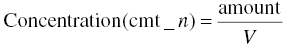
Model predicted concentrations result from dividing the mass amount of drug in a compartment by the volume of distribution, V, of that compartment, or a scaled volume that is discussed here. The mass units of the amount of drug in the nth compartment are the same as the units used to express the dose in the AMT data item in the dataset. In addition, there may be a desire to obtain the estimate of volume in certain units, for example, liters. This can be expressed as follows in Equation 3.1:
If the units of the predicted concentrations are different than those of the dependent variable (DV), that is, the observed concentrations, they must be normalized, or scaled, for the correct computation of residuals during the estimation process. One cannot properly subtract predicted from observed concentrations to compute the residual, if both values are not expressed in the same units.
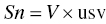
One can define a scale parameter that can be used to normalize the units of the predicted concentrations with the observed concentrations. The scale parameter, Sn, serves to reconcile: (i) the mass units of the dose and concentration values and, simultaneously, (ii) the volume units of the volume of distribution parameter and the units of the observed concentrations. Here n is the compartment number in which the concentrations are observed.
The scale parameter, Sn, is defined as the product of the volume of distribution and a unitless scalar value needed to reconcile the units of predicted and observed concentrations.
For this exercise, let the unitless scalar value be usv as shown in Equation 3.2.
Then,
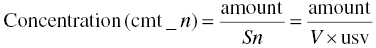
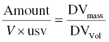
We should define usv, such that when V is replaced by Sn in Equation 3.1, the predicted and observed concentrations have the same units. Thus, the predicted concentration in the nth compartment is as shown in Equation 3.3:
The predicted concentration must have equivalent units to the DV recorded in the DV data item of the dataset. If the concentrations of the observed values are thought of in units of DVmass/DVVol, then the units should be balanced by the following relationship, as shown in Equation 3.4:
Substituting in the units for each term, one may solve for the value of usv.
Consider the following example. Suppose the dose units are mg, the volume of distribution parameter is expressed in L, and the observed concentration units are ng/ml. Then, substituting these values into Equation 3.4, we get:
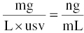
The ng/mL units of DV are 1000 times smaller than mg/L units, so the numerical value of an equivalent concentration is 1000 times larger for ng/mL (e.g., 1 mg/L = 1000 ng/mL). Thus, we need to multiply the left-hand side by 1000 to get the same numerical value in the same units as the right-hand side. The value of usv in this case can be reasoned to be 1/1000, and the $PK code used to implement this scaling would be as shown in Equation 3.6:

Steps to compute this value are also shown here. For this example, starting with Equation 3.5, we wish to use usv to achieve equivalence with ng/mL on the right-hand side of the equation.
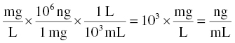
Since we want to express the scale factor in terms of volume, we can rearrange the relationship given earlier to see that:

balances the units of mg × mL/ng.
Here usv = 1/1000, which, when substituted in the $PK expression of the scale parameter Sn, for example, S2 = V2/1000, will normalize the units of predicted and observed concentrations.
This method for determining an appropriate scale factor can be easily applied to situations with differing dose and/or concentration units. It is important to remember, however, that the variable name for the appropriate volume parameter is determined by the ADVAN TRANS combination selected for the model and should be set accordingly.
3.5.2.3 Estimating Interindividual Variability (IIV)
In the Example Partial $PK Block provided in Section 3.5.2.1, an exponential function (i.e., EXP(x) in FORTRAN) is used to introduce IIV on clearance and volume. In terms of the population estimate obtained for the ETA, this model is equivalent to modeling IIV with the constant coefficient of variation (CCV) or proportional error model (described in more detail in Chapter 2) when first-order (i.e., classical) estimation methods are implemented. This is because, when the first-order Taylor series approximation is applied to models using these parameterizations [× (EXP(ETA(x)) and × (1 + ETA(x))], the result is the same. However, the advantage of the exponential function for IIV (over the CCV or proportional function) is that the PK parameter is inherently constrained to be positive if the fixed effects are constrained to be positive. For the simple case, when the typical value of the PK parameter is defined to be an element of THETA with a lower bound of 0, the incorporation of IIV using the exponential notation will always result in a positive value for the subject-specific estimate of the PK parameter, even with extremely small and negative values of ETA(1). On the other hand, with the CCV notation, negative values of ETA(1) may result in a negative individual PK parameter estimate even when the fixed-effect parameter is constrained to be positive. Other options for modeling IIV would be coded as follows:
Additive (homoscedastic or constant variance) model
TVCL = THETA(1)

CL = TVCL + ETA(1)
Note that this parameterization is also subject to the possibility of negative individual parameter values (CLi) when the ETA(1) is negative. This possibility is typically of concern for PK parameters but may be very reasonable for certain PD parameters (e.g., parameters measuring a change from baseline scale which could either increase or decrease). The resulting distribution of individual PK parameter values is normally distributed with the additive model for IIV.
Proportional or constant coefficient of variation (CCV) model
TVCL = THETA(1)

CL = TVCL * (1 + ETA(1))
Similar to the exponential model for IIV, this parameterization results in a log-normal distribution of the individual PK parameter values. Here, the variance is proportional to the square of the typical parameter value.
Logit transform model for adding IIV to parameters constrained between 0 and 1
TVF1 = THETA(1)

TMP = THETA(1) / (1 – THETA(1))

LGT = LOG(TMP)

TRX = LGT + ETA(1)

X = EXP(TRX) / (1 + EXP(TRX))
With this model, the typical value, THETA(1), may be constrained between 0 and 1 (via initial estimates), resulting in TMP being constrained between 0 and +∞, and LGT and TRX being “constrained” between –∞ and +∞. The variable, X (which can be thought of like a probability, but including IIV) is also constrained between 0 and 1, and it is the individual subject estimate of bioavailability, F1.
3.5.2.4 Defining and Initializing New Variables
At times, new variables are required and these may be initialized and defined within the $PK block. It is important to always initialize a new variable, that is, define it to be a certain value prior to any conditional statements which may alter its value for some subjects or conditions, to ensure proper functioning of any code that depends on the values of this variable. A simple way to initialize new variables is to use the type of coding provided in the following example:
NEWVAR = 0

IF (conditional statement based on existing variables(s))

NEWVAR = 1
Some of the more common situations where new variables are required include the following: when a variable needs to be recoded for easier interpretation of a covariate effect or when multiple indicator variables need to be created from a single multichotomous variable. Both of these examples are illustrated as follows.
To recode a gender variable from the existing SEXM (0 = female, 1 = male) to a new variable, SEXF (0 = male, 1 = female), first create and initialize the new variable:
SEXF = 0; | new variable SEXF created and initialized to 0 for all subjects |
IF (SEXM.EQ.0) SEXF = 1 | ; when existing variable SEXM=0 (subject is female), set new variable SEXF equal to 1 |
To create multiple indicator variables for race from a single multichotomous nominal variable (i.e., RACE, where 1 = Caucasian, 2 = Black/African American, 3 = Asian, 4 = Pacific Islander, 5 = Other):
RACB = 0 | ; new variable RACB created and initialized to 0 for all subjects |
IF (RACE.EQ.2) RACB = 1 | ; when existing variable RACE=2 (subject is Black), set new variable RACB=1 |
RACA = 0IF (RACE.EQ.3) RACA = 1RACP = 0IF (RACE.EQ.4) RACP = 1RACO = 0IF (RACE.EQ.5) RACO = 1 | ; etc. |
Note that with this coding method, a total of only n − 1 indicator variables are necessary, where n = the number of levels or categories of the original multichotomous variable. In this case, the original RACE variable had a total of five levels, and four indicator variables (RACB, RACA, RACP, and RACO) were created. A fifth new variable to define race = Caucasian (the only remaining group) is not necessary because this group can be uniquely identified by the new dichotomous variables, when all are = 0; this indicates that the subject is not positive for any of the other categories, and therefore, must be Caucasian. The category without a specific indicator variable is thus, considered the reference group or population for this covariate effect. Although the selection of the particular group to set as the reference can be based on desired interpretability of the parameters, choosing the group with the largest frequency can also be considered a reasonable strategy for model stability and to ensure a reasonable degree of precision of the parameter estimates.
3.5.2.5 IF–THEN Structures
At times, it may be necessary or convenient to define parameters differently for portions of the analysis population. In those situations, it may be useful to code the model using an IF–THEN conditional structure. There are several ways to implement such a structure and several examples follow.


