Unless something disturbs a solution (e.g., extreme solute concentration or temperature), there is normally no reason to fear its stability, aside from potential microbial contamination. It should be remembered that the dissolution process is a dynamic equilibrium, meaning the dynamics of crystallization and solution must be complete, and the solute ‘completely’ in solution, in order for a solution to be useful. During the dissolution process, intermolecular interactions are once again at work. Solute particles attract each other; solvent particles also attract each other (cohesive interactions), but hopefully there is sufficient attraction between solute and solvent particles to favor some, or all, of the solute to dissolve. Arguably, the most important aspect regarding pharmaceutical application of solutions is the total solubility of the solute in the solvent. The next most important aspect is the dissolution rate of the solute in the solvent. For end products it is assumed dissolution is complete. However, when preparing solutions for drug use, the amount of time required for the solution to be ‘ready’ (thus, its dissolution rate) is tantamount, and often dissolution is the rate-limiting step when preparing solutions for drug delivery systems.
Until this point, when ‘solutions’ have been discussed, it has been implied that, once a solute has dissolved into the solvent and a solution created, the solution then behaves in an ideal manner, meaning it could be assumed that physical attributes of the solution, like freezing point, remain the same for the solution. However, once again, intermolecular interactions cause deviations from anticipated behavior, and can affect the successful preparation or administration of various drug delivery systems.
Recall introductory chemistry: it may have been interesting to learn that the properties of freezing point, boiling point and vapor pressure of various substances could be altered by the addition of a second substance – an ‘impurity.’ Perhaps even the property of osmotic pressure, and the effects added solutes have on it, were discussed in this context. These are the four colligative properties of solutions. Colligative properties are those that depend on the number of particles in a solution, not the nature of the particles.
There are extensive and intensive physical properties for substances. Extensive properties include parameters such as mass and volume and depend on the amount, or size, of the substance being measured. Intensive properties include characteristics such as density and concentration, and are characteristics of the specific substance, regardless of how much of the substance is observed. Colligative properties are intensive properties of solutions. A formal definition for a colligative property is that the property depends on the quantity (or concentration) of particles in a solution, but is independent of the identity of the particles.
The colligative properties of a given solution include its vapor pressure, boiling point, freezing point and osmotic pressure. The phenomena associated with addition of solute to solvent are vapor pressure lowering, boiling point elevation, freezing point depression and osmotic pressure elevation (changes). All of these are induced by the added solute and result in deviations from properties of the pure solvent. The colligative property most identifiable with biological consequences is osmotic pressure. However, any colligative property can be used to observe (and also to calculate) the effects of addition of a solute to a solvent, and be equated to the other colligative properties. That is, they all indirectly tell us the same information regarding change in the solution, only they are telling us in different ‘languages.’ What are colligative properties, what causes them, and what are the applications with regard to pharmaceuticals?
Key Point
Colligative property deviations that result from adding solute to pure solvent depend only on the amount of added solute, not what the substance added is.
Colligative properties of liquids are affected by the number of particles (molecules or ions) of the solute added to the liquid and are not dependent on the chemical character of the particles. The difficulty is to accurately account for the number of particles and this is not always as straightforward as it may appear. ‘Particles’ usually refers to molecules or ions. However, it is probably familiar that in many cases, solutes, especially electrolytes, though perhaps completely dissolved (by the definition provided in Chapter 3) are not always completely ionically dissociated. Ionization is an equilibrium process. This is important to us because colligative properties, being dependent on the number of particles in solutions, deviate from ‘ideal’ calculations when potentially ionizable solutes are included in a dosage form, but the deviations differ from what might be expected, even if we know precisely how much solute was added. This affects the quantities of solutes that are actually added to solutions. Thus, solutions we deal with will frequently deviate from ideal expectations and our cursory calculations. Whether deviations will exert enough impact on either the patient or the drug delivery system must be considered when preparing solutions – especially those for parenteral administration. Colligative properties, like many important aspects of drug delivery systems, result from intermolecular interactions, and we will briefly see why for each colligative property. With a little mathematical manipulation, all values can be related to concentration, and therefore number of particles, and so be practically applied to dosage form preparation. A brief overview of the four colligative properties is provided below.
Freezing point depression: By adding solute particles, the solvent is diluted, decreasing solvent–solvent interactions, and, ultimately, crystal formation. In order for the solution to freeze, a lower temperature must be attained than is required for freezing the pure solvent. Freezing point depression (∆Tf) is calculated using the equation:

where Tf = freezing point, Kf is the cryoscopic constant (= 1.86°C kg/mol for water) and m = molality of the solution.
Boiling point elevation: As described above, dissolution of a solute, while increasing the concentration of the solute, can be viewed as diluting the concentration of solvent molecules, as well as establishing attractive forces between solvent and solute molecules. The result is a decreased tendency for solvent molecules to escape, or leave, the solution (i.e., evaporate or boil) compared with pure solvent. Therefore, a higher temperature must be attained by the solution than by the pure solvent in order to boil. Boiling point elevations (∆Tb) are calculated by the equation:

where Kb is the ebullioscopic constant of the solvent (= 0.512°C kg/mol for water).
Vapor pressure depression: As occurs when other colligative properties are explained, dissolving a solute in a solvent decreases the solvent–solvent (cohesive) interactions, while increasing the solvent–solute (adhesive) interactions, resulting, as measured with vapor pressure, in a decreased tendency for solvent molecules to escape the solution, compared with the tendency for pure solvent. Vapor pressure is the force exerted above a liquid (or solid) that results from evaporation of a liquid (or solid) in a closed container. Fewer numbers of solvent molecules vaporizing, by definition, is decreased vapor pressure. Vapor pressure is governed by the parameters included in Raoult’s law:

where PA = solution vapor pressure,  = pure solvent vapor pressure, and XA = mole fraction of solvent.
This shows that addition of a solute, B, to solvent A results in a decreased vapor pressure of solvent A. This form of Raoult’s law focuses on the resulting mole fraction of the solvent but leaves us to further determine the amount of solute that is represented by subtracting from one. The colligative property of vapor pressure depression, resulting from the addition of a solute, B, is really what is of interest. That is, when a solute, XB, is added to a solvent, how much is the vapor pressure decreased? This is simply looking directly at how the quantity of solute affects the solvent. If we know the mole fraction of the solute, XB, then this can be calculated from:

XB will be a unitless fraction, which can then be converted to percent or to Pascals if desired. Therefore, if we are adding a known amount of solute, B, we can estimate what the magnitude of the resulting vapor pressure depression will be.
Osmotic pressure elevation: If a solute is dissolved in a solvent, the solvent’s osmotic pressure is increased. Osmotic pressure is the force applied against a semipermeable membrane by a liquid. Adding solute to the liquid (solvent) can increase that force. If solutes are unable to cross the membrane, but solvents can, osmotic pressure on a membrane can be established, and measured. The lower the concentration of solvent, the higher the osmotic pressure. The higher the solute concentration, the more osmotic pressure is exerted, compared with that of pure solvent. The osmotic pressure of a solution is the difference in pressure between that exerted by the solution versus that of the pure solvent across a semipermeable membrane. In a way, osmotic pressure can be viewed as the resultant force (on the surrounding membrane) applied by a pure solvent, as it proceeds toward equilibrating solute concentration differences. Osmotic pressure change is calculated by the Morse equation:

where R = gas constant, T = absolute temperature, and m = molality of the solution.
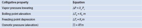
Solutes that completely dissolve and do not ionize (‘simple solutes’) provide straightforward alterations in colligative properties. For these solutions, the four formulae above are accurate. But, what about solutes that have more than one species? These solutes require more attention because if they do not completely ionize, they act partly as the unionized species, but partly as whatever ionizable species may be available. Sometimes the number of species is complicated, and ultimately what is utilized is something of a ‘weighted average’ of each of the ionic forms that are present. But how do we know the proportion of each ionic species? This will be addressed below. A summary of the ideal colligative properties is provided in Table 4.2.
Electrolytes and deviations in colligative properties
Electrolytes are substances that dissolve in water, providing a solution that conducts electricity. An example is sodium chloride:

To begin with, we will assume the ideal condition of 100% dissociation. It will be shown below why the assumption that a solution will behave ideally can lead to puzzling results, especially if the concepts are not understood. The term dissociation, as it is used pertaining to ions, should not be confused with dissociation of particles from a larger solid, as part of the dissolution process. Solutes capable of producing ions that have the capacity to conduct electricity meet the criteria for electrolytes. Electrolytes that are thought to completely (or nearly completely) dissociate are called strong electrolytes. Sodium chloride is a strong electrolyte. Electrolytes that are known to incompletely dissociate are called weak electrolytes. An example of a weak electrolyte is mercury chloride:

Mercury chloride is highly polar but only a small amount (7.4% at 20°C) ionizes in water, meaning the solubility in water is 7.4 g/100 mL. A solution containing mercury chloride does conduct electricity, therefore it is an electrolyte. Keep in mind that dissolution and complete dissociation of ions are two different concepts. Silver chloride is poorly soluble but is a strong electrolyte. Water, as a solvent, does not dissolve a relatively large amount of silver chloride compared to that of sodium chloride. However, of the silver chloride that is dissolved, most of the Ag+ and Cl− completely dissociate from each other. Solutes that dissolve in water but are not fragmented into ions (i.e., maintain their molecular structure in solution), do not conduct electricity and are called nonelectrolytes. An example of a nonelectrolyte is glucose. The dissolution of glucose (C6H12O6) in water:

Key Point
Electrolytes cannot be assumed to dissociate, even if they dissolve. The actual extent of an electrolyte dissociation results in a different number of particles present from the number expected if complete dissociation is assumed.
As a general rule, it may be assumed that most strong electrolytes in solution are actually only about 80% dissociated. The remaining 20% is present in associated forms, such as ion pairs (Figure 4.1). The use of 80% dissociation is a generalization that works for most practical applications. It is emphasized that this is not exact. This ‘rule’ is based on the work of van’t Hoff and others, which is generalized to commonly used electrolytes in pharmaceuticals.
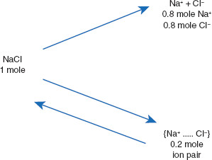
Figure 4.1 Explanation of van’t Hoff i values correction for electrolyte dissociation
van’t Hoff (and others) noted deviations from ideal dissociation could be explained using the concept of ion pairs as a reservoir for a portion of what previously was believed to be dissociated electrolyte. The application was to determine corrected dissociation constants for various electrolytes. These values often are labeled E in tables.
One mole of sodium chloride results in 1.8 moles of particles (Figure 4.1), rather than the predicted two moles. This deviation from expectation will impact the accuracy of calculations pertaining to drug solutions, as will be illustrated below. First, the application of colligative properties to solutions will be reviewed.
Colligative properties applied to pharmaceutical solutions
An example, using freezing point depression is: ‘How much sodium chloride would be required to be added to 100 mL of water to depress the freezing point 0.52°C if the sodium chloride is completely dissociated?’ To begin, the ‘complete dissociation’ of sodium chloride assumption allows for a simple calculation as complete dissociation of sodium chloride provides two particles from the initial one. The value selected for the freezing point depression chosen is significant because this is actually the freezing point of blood. That is, blood exhibits a freezing point depression of 0.52°C compared to water. Why is the freezing point of blood of interest? Because matching colligative actions of pharmaceutical liquids causes them to act in a ‘physiologic’ way with regard to tonicity. Tonicity is the amount of pressure exerted by a fluid against biological membranes. Ultimately, solutions we make for drug delivery systems usually need to be isotonic. Isotonic solutions are those that exert the same (osmotic) pressure against membranes as physiologic liquids do. Usually, the liquid we attempt to ‘match’ is the tonicity of blood. As mentioned previously, though it may initially seem odd to be associating freezing point with tonicity/osmotic pressure, all four colligative properties are interchangeable, and thus the inference of equivalence among them with regard to tonicity effects on solutions; therefore, the significance of matching the colligative effects exerted by biological fluids (e.g., cells) and so the significance of the ‘standard’ freezing point depression of 0.52°C. This is straightforward as 100% dissociation will be assumed for now:
m is the molal concentration, moles of solute per kg of solvent; 1.86° is the cryoscopic constant for water.
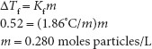
The result of calculating how much sodium chloride causes water to behave like blood in a colligative sense, results in ‘0.280 moles of particles per liter.’ The implication is that it does not matter what the ‘particles’ actually are, just that they are in solution. If so, then 0.280 moles/L (280 mM) is a ‘standard’ for any solute in water, if we want the solution to behave like blood, with regard to osmotic pressure. Therefore, 0.280 moles of any particles/L provides ‘physiologic osmotic pressure.’ This is the concentration of particles in physiological fluids, and so the ideal for parenteral medication solutions.
0.280 moles/L (280 mmol/L) of any solute, or combination of solutes, is considered isotonic.
Stay updated, free articles. Join our Telegram channel

Full access? Get Clinical Tree


