A large amount of in silico research worldwide has been oriented toward the rational drug discovery, property prediction, toxicity, and risk assessment of new drug molecules, as well as chemicals [1]. Quantitative structure–activity relationship (QSAR) analysis has gained great popularity recently in order to fulfill the following objectives [2]: (a) prediction of new analogs with better activity; (b) improved understanding and investigation of the mode of action of chemicals and pharmaceuticals; (c) optimization of the lead compound to congeners with decreased toxicity; (d) rationalization of wet laboratory experimentation (QSAR offers an economical and time-effective alternative to the medium-throughput in vitro and low-throughput in vivo assays); (e) reduction of cost, time, and manpower requirements by developing more effective compounds using a scientifically less exhaustive approach; and finally, (f) to develop alternative methods to animal experimentation in conformity to the Registration, Evaluation, and Authorization of Chemicals (REACH) guidelines [3] and the 3R concept [4], which signifies “reduction, replacement, and refinement” of animal experiments. As a consequence, the QSAR technique emerges as an alternative tool to use for the design, development, and screening of new drug molecules and chemical substances.

The QSAR models are principally applied to predict the activity/property/toxicity of new classes of compounds falling within the domain of applicability of the developed models. Again, to check the acceptability and reliability of the QSAR models’ predictions, validation of the QSAR model has been recognized as one of the key elements [5]. It is now accepted that validation is a more holistic process for assessing the quality of data, applicability, and mechanistic interpretability of the developed model [6]. Various methodological aspects of validation of QSARs have been the subject of much debate within the academic and regulatory communities. The following questions are often raised before successful validation and succeeding appliance of a QSAR model:

The Organisation for Economic Cooperation and Development (OECD) [7] has agreed to five principles that should be followed to set up the scientific validity of a QSAR model, thereby facilitating its recognition for regulatory purposes. OECD principle 4 refers to the need to establish “appropriate measures of goodness-of-fit, robustness, and predictivity” for any QSAR model. It identifies the need to validate a model internally (as represented by goodness-of-fit and robustness) as well as externally (predictivity). Validation strategies largely depend on various metrics. The statistical quality of regression- and classification-based QSAR models can be examined by different statistical metrics developed over the years [8].

Another important aspect of the validation of the QSAR model is the need to define an applicability domain (AD)—that is, OECD principle 3—of the developed QSAR model. The AD expresses the fact that QSARs are inescapably associated with restrictions in the categories of chemical structures, physicochemical properties, and mechanisms of action for which the models can generate reliable predictions [9]. The AD of a QSAR model has been defined as the response and chemical structure space, characterized by the properties of the molecules in the training set. The developed model can predict a new molecule confidently only if the new compound lies in the AD of the QSAR model. It is extremely helpful for the QSAR model user to have information about the AD of the developed model to identify interpolation (true prediction) or extrapolation (less reliable prediction) [10].

Bearing in mind the magnitude of QSAR validation approaches and different validation parameters in the development of successful and acceptable QSAR models, this chapter will focus on classical as well as relatively new validation metrics used to judge the quality of the QSAR models. Along with the validation metrics, the important concepts of the AD approach to build reliable and acceptable QSAR models are discussed thoroughly.

With the introduction of fast computational approaches, it is now feasible to calculate a large number of descriptors using various software tools. However, one cannot ignore the risk of chance correlations with the increased number of variables included in the final model as compared to the number of compounds for which the model is constructed [11]. Again, employing diverse optimization procedures, it is possible to obtain models that can fit the experimental data well, but there is always a chance of overfitting. Fitting of data does not confirm the predictability of a model, as it does for the quality of the model. This is the main basis behind the necessity of validation of the developed models in terms of robustness and predictivity. A QSAR model is fundamentally judged in terms of its predictivity; that is, representing how well it is able to forecast end-point values of molecules that are not employed to develop the correlation.

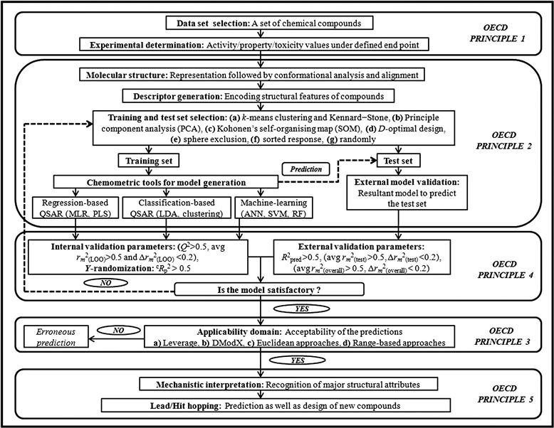
Apart from the use of fitness parameters to judge the statistical quality of the model, validation of QSAR models is carried out using two major strategies [12]: (i) internal validation using the training set molecules, and (ii) external validation based on the test set compounds by splitting the whole data set into training and test sets. However, there is another technique called true external validation, which uses the developed QSAR model to predict an external data set. It is important to mention that many times, an external data set is absent for the same end point. In such a case, the data set is divided into a training and a test set for external validation. Here, for better understanding of the validation methods, we are including true external validation in the discussion of the basic external validation approach. Both the internal and external validation methods have been considered by different groups of researchers for evaluating the predictability of the models. Besides these techniques, randomization or Y-scrambling (again, which can be regarded as a type of internal validation) executed on the data matrix provides a valuable technique for evaluating the existence of any chance correlation in the QSAR model. Along with these validation techniques, determination of the AD of the model and selection of outliers are other vital aspects in the course of developing a reliable QSAR model with the spirit of OECD principles. The steps for development of reliable and acceptable QSAR model along with the currently employed validation methods are demonstrated in Figure 7.1.

7.2.3 External validation

Internal validation considers only chemicals belonging to the same set of compounds. As a consequence, one cannot judge the predictive capability of the developed model when it has been employed to predict a completely new set of compounds. In many cases, where truly external data points are unavailable for prediction purposes, the original data set compounds are divided into training and test sets [18], thus enabling external validation. This subdivision of the data set can be accomplished in many ways. The details about the division of the data set into training and test sets are illustrated in Section 7.2.3.1. In the case of external validation, the data set is initially divided into training and test sets, and subsequently, a model is developed with the training set and the constructed model is employed to check the external validation by utilizing the test set molecules that are not used in the model development process. The external validation ensures the predictability and applicability of the developed QSAR model for the prediction of untested molecules. A series of both classical and newly introduced validation metrics and model stability parameters are discussed in Section 7.2.4.

7.2.3.1 Division of the data set into training and test sets

The selection of training and test sets should be based on the immediacy of the test set members to representative points of the training set in the multidimensional descriptor space [19,20]. Ideally, this division must be performed such that points representing both training and test sets are distributed within the whole descriptor space occupied by the whole data set and each point of the test set is near at least one compound of the training set. This approach ensures that the similarity principle can be employed for the activity prediction of the test set [19]. There are several possible approaches available for the selection of the training and test sets. The following approaches are largely employed by the QSAR practitioners:

i. Random selection: In this method, the data set is divided into training and test sets by a mere random selection.

ii. Based on Y-response: One more frequently used approach is based on the activity (Y-response) sampling. The whole range of activities is divided into bins, and compounds belonging to each bin are randomly (or in some regular way) assigned to the training or test sets [21].

iii. Based on X-response: Another approach is selection of the training and test sets on the basis of compound similarity. In this method, physicochemical properties and structural similarity of the compounds are considered for the grouping of similar or homologous compounds. Thereafter, a predecided portion of compounds is manually or in some regular way assigned to the training or test set.

The test set thus selected may vary in size depending upon the number of compounds in the data set. The selection of molecules in the training and test sets, as well as their size, are the prime criteria for development of a statistically significant QSAR model [22]. From this perspective, the most generally employed tools for rational division of the data set into training and test sets are discussed in the following list:

a. k-Means clustering: The k-means clustering is one of the best known nonhierarchical clustering techniques [23]. This approach is based on clustering a series of compounds into several statistically representative classes of chemicals. At the end of the analysis, the data are split into k clusters. As the result of k-means clustering analysis, one can examine the means for each cluster on each dimension to assess how distinct the k clusters are. This procedure ensures that any chemical class is represented in both series of compounds (i.e., training and test sets) [23].

b. Kohonen’s self-organizing map selection: Kohonen’s self-organizing map (SOM) considers the closeness between data points. One has to remember that these points, which are close to each other in the multidimensional descriptor space, are also close to each other on the generated map by the SOM. Representative points falling into the identical areas of the SOM are arbitrarily chosen for the training and test sets. The shortcoming of this method is that the quantitative methods of prediction use accurate values of distances between representative points: as SOM is a nonlinear projection method, the distances between points in the map are distorted [24].

c. Statistical molecular design: Statistical molecular design may be employed for the training set selection [25]. It uses a large number of molecular structures for which the response variable (Y) is not required. Molecular descriptors are computed for all compounds, and principal component analysis (PCA) is performed. The principal components (PCs) that are combinations of the molecular properties signify the principal properties of the data set explaining the variation among the molecules in an optimal way. The design is then executed with respect to the principal properties by picking a subset of compounds that are most competent in spanning the substance space and, thus, are the best selection of training set for a QSAR model. The selection can be done manually from the score plots if the number of PCs is less than 3 or 4 [26].

d. Kennard–Stone selection: To pick a representative subset from a data set, hierarchical clustering and maximum dissimilarity approach also can be employed. The Kennard–Stone method selects a subset of samples from N that offers unvarying coverage over the data set and includes samples on the boundary of the data set. The method begins by finding the two samples that are farthest apart in terms of geometric distance. To add another sample to the selection set, the algorithm selects from the remaining samples the one that has the greatest separation distance from the selected samples. The separation distance of a candidate sample from the selected set is the distance from the candidate to its closest selected sample. This most-separated sample is then added to the selection set, and the process is repeated until the required number of samples, x, has been added to the selection set. The drawbacks of clustering methods are that different clusters contain different numbers of points and have different densities of representative points. Therefore, the closeness of each point of the test set to at least one point of the training set is not guaranteed. Maximum dissimilarity and Kennard–Stone methods guarantee that the points of the training set are distributed more or less evenly within the whole area occupied by representative points, and the condition of closeness of the test set points to the training set points is satisfied [27].

e. Sphere exclusion: In the sphere exclusion method, a compound with the highest activity is selected and included in the training set. A sphere with the center in the representative point of this compound with radius r=d(V/N)^1/P is built, where P is the number of variables that represents the dimensionality of descriptor space, d is the dissimilarity level, N is the total number of compounds in the data set, and V is the total volume occupied by the representative points of compounds. The dissimilarity level is varied to create different training and test sets. The molecules corresponding to representative points within this sphere (except for the center) are incorporated in the test set. All points within this sphere are excluded from the initial set of compounds. Let n be the number of remaining compounds. If n=0, splitting is stopped [28]. If n>0, the next compound is randomly selected. Otherwise, distances of the representative points of the remaining compounds to the sphere centers are calculated, and a compound with the smallest or greatest distance is selected.

f. Extrapolation-oriented test set selection: Extrapolation-oriented test set selection is an external validation method that performs better than those constructed by random selection and uniformly distributed selection. This algorithm selects pairs of molecules from those available that have the highest Euclidean distance in the descriptor space and then moves them to the external validation set, one after the other, until the set is complete [29].

The OECD members did not prepare any general rules regarding the impact of training and test set size on the quality of prediction, but it is important to point out that the training set size should be set at an optimal level so that the model is developed with a reliable and acceptable number of training set compounds and it is able to satisfactorily predict the activity values of the test set compounds. Note that the division of a data set using some common algorithms can be easily done by the use of an open-access tool called Dataset Division GUI 1.0, available at http://dtclab.webs.com/software-tools and http://teqip.jdvu.ac.in/QSAR_Tools/.

7.2.3.2 Applicability domain

7.2.3.2.1 Concept of the AD

The AD [30] is a theoretical region in the chemical space surrounding both the model descriptors and modeled response. In the construction of a QSAR model, the AD of molecules plays a deciding role in estimating the uncertainty in the prediction of a particular compound based on how similar it is to the compounds used to build the model. Therefore, the prediction of a modeled response using QSAR is applicable only if the compound being predicted falls within the AD of the model, as it is impractical to predict an entire universe of chemicals using a single QSAR model. Again, AD can be described as the physicochemical, structural, or biological space information based on which the training set of the model is developed, and the model is applicable to make predictions for new compounds within the specific domain [31].

One has to remember that the selection process of the training and test sets has a very important effect on the AD of the constructed QSAR model. Thus, while splitting a data set for external validation, the training set molecules should be selected in such a way that they span the entire chemical space for all the data set molecules. In order to obtain successful predictions, a QSAR model should always be used for compounds within its AD.

7.2.3.2.2 History behind the introduction of the AD

A QSAR model is essentially valued in terms of its predictability, indicating how well it is able to predict the end-point values of the compounds that are not used to develop the correlation. Models that have been validated internally and externally can be considered reliable for both scientific and regulatory purposes [32]. As decided by the OECD, QSAR models should be validated according to the OECD principles for reliable predictions (elaborated previously in this chapter in Section 7.2.1). Thus, the present challenge in the procedure of developing a QSAR model is no longer ensuring that the model is statistically able to predict the activity within the training set, but developing a model that can predict accurately the activity of untested chemicals.

In this context, QSAR model predictions are most consistent if they are derived from the model’s AD, which is broadly defined under OECD principle 3. The OECD includes AD assessment as one of the QSAR acceptance criteria for regulatory purposes [14]. The Setubal Workshop report [13] presented the following regulation for AD assessment: “The applicability domain of a (Q)SAR is the physicochemical, structural, or biological space, knowledge, or information on which the training set of the model has been developed, and for which it is applicable to make predictions for new compounds. The applicability domain of a (Q)SAR should be described in terms of the most relevant parameters, i.e. usually those that are descriptors of the model. Ideally the (Q)SAR should only be used to make predictions within that domain by interpolation not extrapolation.” This depiction is useful for explaining the instinctive meaning of the “applicability domain” approach.

7.2.3.2.3 Types of AD approaches

The most common approaches for estimating interpolation regions in a multivariate space include the following [10]:

• Ranges in the descriptor space

• Geometrical methods

• Distance-based methods

• Probability density distribution

• Range of the response variable

The first four approaches are based on the methodology used for interpolation space characterization in the model descriptor space. The last one, however, depends solely on the response space of the training set molecules. A compound can be identified as being out of the domain of applicability in a simple way; namely, (a) at least one descriptor is out of the span of the ranges approach and (b) the distance between the chemical and the center of the training data set exceeds the threshold for distance approaches. The threshold for all kinds of distance methods is the largest distance between the training set data points and the center of the training data set. Classification of the AD approaches is graphically presented in Figure 7.2. In order to better explain the theory, criteria, and drawbacks of each type of AD approaches [9,10,30,33–48], we have depicted all the methods in Table 7.1.

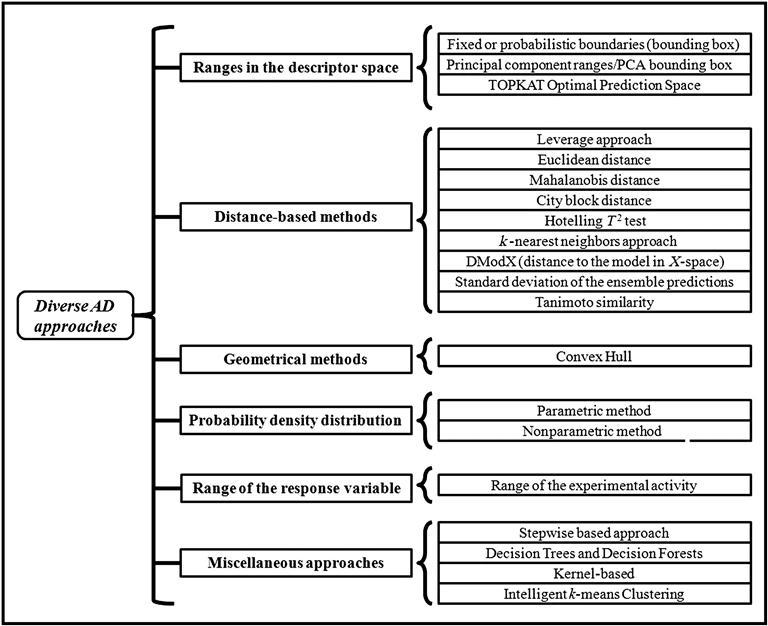
Table 7.1

Hypotheses of diverse AD methods

Types	Subtypes	Theory, criteria, and drawbacks, if any	Reference
Ranges in the descriptor space approach	Fixed or probabilistic boundaries/bounding box	Theory: The ranges of the each descriptor are considered with a uniform distribution defining an n-dimensional hyper-rectangle developed on the basis of the highest and lowest values of individual descriptors employed to construct the model with sides parallel to the coordinate axes.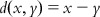 d(x,y)=x−y	[33]
		Criteria: The boundary is generated based on the highest and lowest values of X variables (descriptors to develop the model) and Y variable (response for which the QSAR equation is formed) of the training set. Any test set compounds that are not present in any of these particular ranges are considered outside the AD, and their predictions are less reliable.
		Drawbacks: (a) Due to nonuniform distribution, the method encloses substantial empty space; (b) empty regions in the interpolation space cannot be predictable, as only the descriptor ranges are considered; (c) correlation between descriptors cannot be taken into account.
	PC ranges/PCA bounding box	Theory: Principal components convert the original data into a new orthogonal coordinate system by the rotation of axes and facilitate to correct for correlations among descriptors. Newly formed axes are defined as PCs presenting the maximum variance of the total compounds. The points between the lowest value and the highest value of each PC define an n-dimensional (n is the number of significant components) hyper-rectangle with sides parallel to the PCs.	[33,34]
		Criteria: This hyper-rectangle AD also includes empty spaces depending on uniformity of data distribution. Combining the bounding box method with PCA can overcome the setback of correlation between descriptors, but the issue of empty regions within the interpolation space remains. It is interesting to point out that the empty space is smaller than the hyper-rectangle in the original descriptor ranges.
	TOPKAT optimal prediction space	Theory: A variation of PCA is implemented by the optimum prediction space (OPS) from TOPKAT OPS 2000. In the PCA approach, instead of the standardized mean value, the data is centered around the mean of individual parameter range ([xmax–xmin]/2). Thus, it establishes a new orthogonal coordinate system which is known as OPS coordinate system. Here, the basic process is the same, extracting eigenvalues and eigenvectors from the covariance matrix of the transformed data. The OPS boundary is defined by the minimum and maximum values of the generated data points on each axis of the OPS coordinate system.	[35]
		Criteria: The property sensitive object similarity (PSS) is implemented in the TOPKAT as a heuristic solution to replicate the the data set’s dense and spare regions, and it includes the response variable (y). Accuracy of prediction between the training set and queried points is assessed by the PSS. Similarity, a search method is used to evaluate the performance of TOPKAT in predicting the effects of a chemical that is structurally similar to the training structure.
Geometrical methods	Convex hull	Theory: This estimates the direct coverage of an n-dimensional set employing convex hull calculation, which is performed based on complex but efficient algorithms. The approach recognizes the boundary of the data set considering the degree of data distribution.	[33,36]
		Criterion: Interpolation space is defined by the smallest convex area containing the entire training set.
		Drawbacks: (a) Implementing a convex hull can be challenging, as an increase in dimensions contributes to the order of complexity. Convex hull calculation is efficient for two and three dimensions. The complexity swiftly amplifies in higher dimensions. For n points and d dimensions, the complexity is of order O, which can be defined as O=[n[d/2]+1]. (b) The approach only analyzes the set boundaries without considering the actual data distribution. (c) It cannot identify the potential internal empty regions within the interpolation space.
Distance-based methods (based on the distance-to-centroid principle)	Leverage approach	Theory: The leverage (h) of a compound in the original variable space is calculated based on the HAT matrix as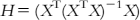 H=(XT(XTX)−1X) where H is an [n×n] matrix that orthogonally projects vectors into the space spanned by the columns of X. The AD of the model is defined as a squared area within the ±3 band for standardized cross-validated residuals (σ), and the leverage threshold is defined as h*=3(p+1)/n, where p is the number of variables and n is the number of compounds. The leverage values (h) are calculated (in the X-axis) for each compound and plotted versus cross-validated standardized residuals (σ) (in the Y-axis), referred to as the Williams plot.	[30,37]
		The leverage approach assumes normal data distribution. It is interesting to point out that when high leverage points fit the model well (having small residuals), they are called good high leverage points or good influence points. Those points stabilize the model and make it more accurate. On the contrary, high leverage points, which do not fit the model (having large residuals), are called bad high leverage points or bad influence points.
		Criteria: The Williams plot confirms the presence of response outliers (when the compound bears a standardized cross-validated residual value greater than ±3σ units, but it lies within the critical HAT [h*]) and training set chemicals that are structurally very influential (higher leverage value than h*, but lie within the fixed ±3σ limit of the ordinate) in determining model parameters. It is interesting to point out that although the chemical is influential one for the model, it is not a response outlier (not a Y outlier). The data predicted for high leverage chemicals in the prediction set are extrapolated and could be less reliable.
	Euclidean distance	Theory: This approach calculates the distance from every other point to a particular point in the data set. A distance score, dij, for two different compounds Xi and Xj can be measured by the Euclidean distance norm. The Euclidean distance can be expressed by the following equation: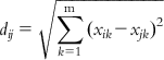 dij=∑k=1m(xik−xjk)2	[38]
		The mean distances of one sample to the residual ones are calculated as follows: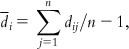 d¯i=∑j=1ndij/n−1, where i=1,2,…,n.
		The mean distances are then normalized within the interval of zero to 1. It is applicable only for statistically independent descriptors.
		Criteria: Compounds with distance values adequately higher than those of the most active probes are considered to be outside the domain of applicability. The mean normalized distances are measured for both training and test set compounds. The boundary region created by normalized mean distance scores of the training set are considered as the AD zone for test set compounds. If the test set compounds are inside the domain, then these compounds are inside the AD; otherwise, they are not.
	Mahalanobis distance	Theory: The approach considers the distance of an observation from the mean values of the independent variables, but not the impact on the predicted value. It offers one of the distinctive and simple approaches for identification of outliers. The approach is unique because it automatically takes into account the correlation between descriptor axes.	[39]
		Criterion: Observations with values much greater than those of the remaining ones may be considered to be outside the domain.
	City block distance	City block distance is the summed difference across dimensions and is computed employing the following equation: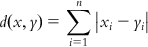 d(x,y)=∑i=1n|xi−yi|	[38]
		It examines the complete differences between coordinates of a pair of objects (xi and yi) and it assumes a triangular distribution. The method is predominantly useful for the distinct type of descriptors. It is used only for training sets that are uniformly distributed with respect to count-based descriptors.
	Hotelling T2 test	Theory: The Hotelling T2 method is a multivariate student’s t test and proportional to leverage and Mahalanobis distance approach. It presumes a normal data distribution like the leverage approach. The method is used to evaluate the statistical impact of the difference on the means of two or more variables between two groups. Hotelling T2 corrects for collinear descriptors through the use of the covariance matrix. Hotelling T2 measures the distance of an observation from the center of a set of X observations. A tolerance volume is derived for Hotelling T2.	[39]
		Criterion: Based on the t value, the significant compounds within the domain are determined.
	k-nearest neighbors approach	Theory: The approach is based on a similarity search for a new chemical entity with respect to the space shaped by the training set compounds. The similarity is identified by finding the distance of a query chemical from the nearest training compound or its distances from k-nearest neighbors in the training set. Thus, similarity to the training set molecules is significant for this approach in order to associate a query chemical with reliable prediction.	[40]
		Criterion: If the calculated distance values of test set compounds are within the user-defined threshold set by the training set molecules, then the prediction of these compounds are considered to be reliable.
	DModX (distance to the model in X-space)	Theory: This approach is usually applied for the partial least squares (PLS) models. The basic theory lies in the residuals of Y and X, which are of diagnostic value for the quality of the model. As there are a number of X-residuals, one needs a summary for each observation. This is accomplished by the residual standard deviation (SD) of the X-residuals of the corresponding row of the residual matrix E. As this SD is proportional to the distance between the data point and the model plane in X-space, it is usually called DModX (distance to the model in X-space). Here, X is the matrix of predictor variables, of size (N*K); Y is the matrix of response variables, of size (N*M); E is the (N*K) matrix of X-residuals; N is number of objects (cases, observations); k is the index of X-variables (k=1, 2, …, K); and m is the index of Y-variables (m=1, 2,…, M).	[9,41]
		Criteria: A DModX value larger than around 2.5 times the overall SD of the X residuals (corresponding to an F-value of 6.25) signifies that the observation is outside the AD of the model. In the DModX plot, the threshold line is attributed as a D-critical line, and this plot can be drawn in SIMCA-P software.
	Tanimoto similarity	The Tanimoto index measures similarity between two compounds based on the number of common molecular fragments. In order to calculate the Tanimoto similarity, all single fragments of a particular length in two compounds are computed. The Tanimoto similarity between the compounds J and I is defined as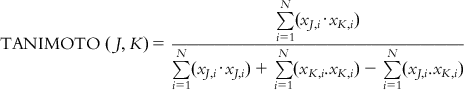 TANIMOTO(J,K)=∑i=1N(xJ,i⋅xK,i)∑i=1N(xJ,i⋅xJ,i)+∑i=1N(xK,i.xK,i)−∑i=1N(xJ,i.xK,i) < div class='tao-gold-member'> Only gold members can continue reading. Log In or Register to continue Share this: Click to share on Twitter (Opens in new window) Click to share on Facebook (Opens in new window) Like this: Like Loading... Related Related posts: Future Avenues Introduction to 3D-QSAR Other Related Techniques Selected Statistical Methods in QSAR Stay updated, free articles. Join our Telegram channel Join Tags: Understanding the Basics of QSAR for Applications in Pharmaceutic Jul 18, 2016 | Posted by admin in PHARMACY | Comments Off on Validation of QSAR Models Full access? Get Clinical Tree Get Clinical Tree app for offline access Get Clinical Tree app for offline access %d