Selected Statistical Methods in QSAR
Quantitative structure–activity relationships (QSARs) are predictive statistical models correlating one or more piece of response data about chemicals, with the information numerically encoded in the form of descriptors. Various statistical tools, including regression and classification-based strategies, are used to analyze the response and chemical data and their relationship. Machine learning tools are also very effective in developing predictive models, particularly when handling high-dimensional and complex chemical data showing a nonlinear relationship with the responses of the chemicals. Some of the selected statistical tools commonly used in QSAR studies are briefly discussed in this chapter.
Keywords
Chemometric tools; model development; multiple linear regression (MLR); partial least squares (PLS); linear discriminant analysis (LDA); artificial neural network (ANN)
6.1 Introduction
Quantitative structure–activity relationship (QSAR) models are developed using one or more statistical model building tools, which may be broadly categorized into regression- and classification-based approaches. Machine learning methods, which use artificial intelligence, may also be useful for predictive model development. Note that the latter may also be used for regression and classification problems. Apart from model development, statistical methods are needed for feature selection from a large pool of computed descriptors. As QSAR is a statistical approach, there should be a number of rigorous tests for checking the reliability of the developed models, which may otherwise be proved to be a statistical nuisance if proper care is not taken at every step of its development.
6.2 Regression-Based Approaches
Regression-based approaches are used when both the response variable and independent variables are quantitative. The generated regression model can compute quantitative response data from the model.
6.2.1 Multiple linear regression
Multiple linear regression (MLR) [1] is one of the most popular methods of QSAR due to its simplicity in operation, reproducibility, and ability to allow easy interpretation of the features used. This is a regression approach of the dependent variable (response property or activity) on more than one descriptor. The generalized expression of an MLR equation is as follows:
 (6.1)
(6.1) In Eq. (6.1), Y is the response or dependent variable; X1, X2, … , Xn are descriptors (features or independent variables) present in the model with the corresponding regression coefficients a1, a2, … , an, respectively; and a0 is the constant term of the model.
6.2.1.1 Model development
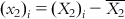
Now consider the method for development of an MLR equation using the least squares method. Say that we have a set of m observations of n descriptors and the corresponding Y values (Table 6.1).
Table 6.1
| Compound No. | Response (Y) | Descriptor 1 (X1) | Descriptor 2 (X2) | Descriptor 3 (X3) | … | Descriptor n (Xn) |
| 1 | (Y)1 | (X1)1 | (X2)1 | (X3)1 | … | (Xn)1 |
| 2 | (Y)2 | (X1)2 | (X2)2 | (X3)2 | … | (Xn)2 |
| 3 | (Y)3 | (X1)3 | (X2)3 | (X3)3 | … | (Xn)3 |
| 4 | (Y)4 | (X1)4 | (X2)4 | (X3)4 | … | (Xn)4 |
 |  |  |  |  |  |  |
| m | (Y)m | (X1)m | (X2)m | (X3)m | … | (Xn)m |
If we want to develop an MLR equation from this data set, then in the ideal case, the developed model should fit the data in a perfect way for all the observations. This means that the calculated Y value (Ycalc) for a particular observation from the model should be exactly the same as the corresponding observed Y value (Yobs).
Thus, in the ideal case, for compound 1,
 (6.2-1)
 Similarly,
 (6.2-2)
 (6.2-m)
 In reality, however, there will be some difference between the observed and calculated response values for most (if not all) of the observations. The objective of the model development should be to minimize this difference (or the residual). However, some of the compounds (observations) will have positive residuals, and others will have negative residuals. Thus, squared residuals are considered while defining the objective function of the model development, which is actually the sum of the squared residuals [Σ(Yobs−Ycalc)2] for all the observations used in the model development; if the model is good, this should attain a low value. Hence, the method is also known as the method of least squares.
Now, while considering a problem such as MLR model development, the unknowns are a0, a1, a2, a3, …, an, while X1, X2, X3,…Xn, and Y are all known quantities. The constant a0 can be easily found once the regression coefficients a1, a2, a3…, an are known. Hence, here we have n unknowns. In case of solution of simultaneous equations, we would have needed only n equations (n observations). However, in our problem, a “perfect solution” is not desired as we must consider that errors are inherent in the biological measurements which will affect the “solutions.” Hence, we adopt a statistical approach of regression, which uses the information from as many observations as possible to give an overall reflection of the contribution of each feature to the response. Equations (6.2-1)–(6.2-m) may be summed to give the following equations:
 (6.3)
(6.3) Dividing both sides of Eq. (6.3) with the number of observations m, we get
 (6.4)
(6.4) If we subtract Eq. (6.4) from each of Eqs. (6.2-1)–(6.2-m), we will get a series of equations with the centered values of the response and descriptors:
 (6.5-1)
  (6.5-2)
  (6.5-3)
 (6.5-m)
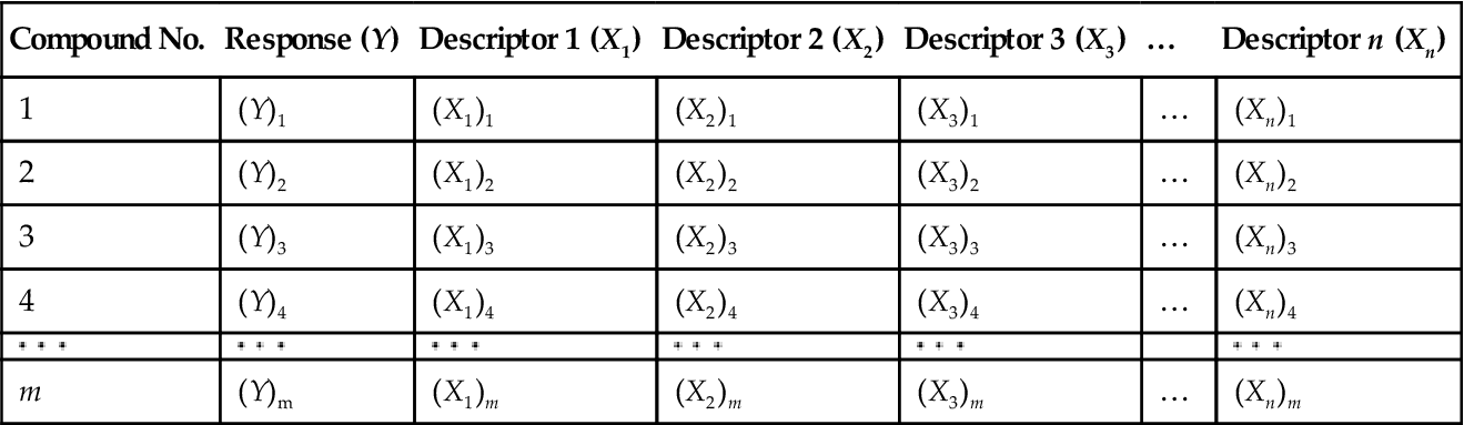
 such that  ,
, 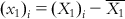 ,
,  ,
,  , etc.
Now, multiplying each of Eqs. (6.5-1)–(6.5-m) by the x1 term of the corresponding observation, we get
 (6.6-1)
  (6.6-2)
  (6.6-3)
 (6.6-m)
 Summing the respective terms in Eqs. (6.6-1)–(6.6-m),
 (6.7-1)
 Similarly, multiplying each of Eqs. (6.5-1)–(6.5-m) with the x2 term of the corresponding observation and then summing the obtained equations, we have
 (6.7-2)
 In a similar manner, we can have
 (6.7-3)
 (6.7-n)
 Equations (6.7-1)–(6.7-n) are called normal equations. These equations are now used to solve the values for n unknowns, a1 to an. Note that each of these normal equations contains information from all m observations, and hence this method of solving is not heavily affected by the possible error in the response value of a particular observation.
In a matrix notation, the problem may now be denoted as follows:
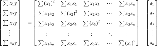
Let us call these three matrices U, V, and W, respectively. Note that the matrix V is a square and symmetric matrix of dimension n (which is equal to the number of unknowns), while the matrices U and W are columns of n rows, n being the number of unknowns. Thus, as the number of unknowns (regression coefficients of descriptors) increases, the complexity of calculation also increases.
The unknown matrix W can be computed by inverting the matrix V and then multiplying by U:
 (6.8)
(6.8) A matrix can be inverted by the Gauss–Jordan method, where elementary operations are applied to both the matrix to be inverted and a unit matrix with the same dimensions such that the matrix to be inverted becomes a unit matrix. With the same sets of elementary operations, the original unit matrix becomes the inverted V matrix (V−1). The matrix V−1 is then multiplied by U. Note that the dimension of V−1 is  , while that of U is
  . Thus, on multiplication, we get a matrix of dimension
  , which is actually the matrix W containing n unknowns (a1, a2, a3, … , an). Once the values of the regression coefficients are known, one can use Eq. (6.4) to calculate the value of a0.
With all the unknowns being known, one can compute the response values (Ycalc) for all the observations and can also check the residual values (Yobs–Ycalc) in order to examine the quality of fits. The analysis of residuals can also identify the outliers, which are different from the rest of the data. A compound having a residual value that lies more than three standard deviations from the mean of the residuals may be considered an outlier. If a residual plot shows that all or most of the residuals are on one side of the 0 residual line, the residuals vary regularly with increasing measured values, or both, it indicates a systemic error. It is also possible to graphically plot the observed experimental values against the calculated values, and the degree of scatter (deviation from the 45° line) will be a measure of lack of fit (LOF). Now, the model having been developed, it is necessary to check the quality of the developed models using different criteria.
6.2.1.2 Statistical metrics to examine the quality of the developed model
6.2.1.2.1 Mean average error
Mean average error (MAE) can be easily determined from the following expression:
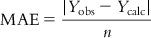 (6.9)
(6.9)where n is the number of observations. Obviously, the value of MAE should be low for a good model. However, the MAE value will largely depend on the unit of the Y observations.
6.2.1.2.2 Determination coefficient (R2)
In order to judge the fitting ability of a model, we can consider the average of the observed Y values ( ) as the reference, such that the model performance should be more than
  . For a good model, the residual values (or the sum of squared residuals) should be small, while the deviation of most of the individual observed Y values from
  is expected to be high. Thus, the ration
 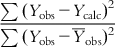 should have a low value for a good model. We can define the determination coefficient (R2) in the following manner:
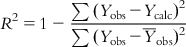 (6.10)
For the ideal model, the sum of squared residuals being 0, the value of R2 is 1. As the value of R2 deviates from 1, the fitting quality of the model deteriorates. The square root of R2 is the multiple correlation coefficient (R).
6.2.1.2.3 Adjusted R2 (R a 2  )
)
If we examine the expression of the determination coefficient, we can see that it only compares the calculated Y values with the experimental ones, without considering the number of descriptors in the model. If one goes on increasing the number of descriptors in the model for a fixed number of observations, R2 values will always increase, but this will lead to a decrease in the degree of freedom and low statistical reliability. Thus, a high value of R2 is not necessarily an indication of a good statistical model that fits the available data. If, for example, one uses 100 descriptors in a model for 100 observations, the resultant model will show R2=1, but it will not have any reliability, as this will be a perfectly fitted model (a solved system) rather than a statistical model. For a reliable model, the number of observations and number of descriptors should bear a ration of at least 5:1. Thus, to better reflect the explained variance (the fraction of the data variance explained by the model), a better measure is adjusted R2, which is defined in the following manner:
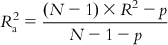 (6.11)
In Eq. (6.11), p is the number of predictor variables used in model development. For a model with a given number of observations (N), as the number of predictor variables increases, the value of R2 increases, while the adjusted R2 value is penalized due to an increase in the number of predictor variables.
6.2.1.2.4 Variance ratio (F)
In an MLR model, the deviations of Y from the population regression plane have mean 0 and variance σ2, which can be shown by the following expression:
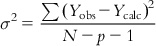 (6.12)
The sum of squares of deviations of the Y from their mean  can be split into two parts: (i) the sum of squares of deviations of the fitted values from their mean
  , with the corresponding degree of freedom being the number of predictor variables (source of variation being regression); and (ii) the sum of squares of deviations of the fitted values from the observed ones
  with the corresponding degree of freedom of N−p−1 (with the source of variations being deviations). To judge the overall significance of the regression coefficients, the variance ratio (the ratio of regression mean square to deviations mean square) can be defined as
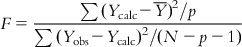 (6.13)
The F value has two degrees of freedom: p and N−p−1. The computed F value of a model should be significant at p<0.05. For overall significance of the regression coefficients, the F value should be high.
The F value also indicates the significance of the multiple correlation coefficient R, and they are related by the following expression:
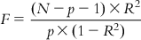 (6.14)
6.2.1.2.5 Standard error of estimate (s)
For a good model, the standard error of estimate of Y should be low, which is defined as
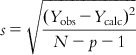 (6.15)
Stay updated, free articles. Join our Telegram channel

Full access? Get Clinical Tree


