Multivariable Analysis

13 Multivariable Analysis


I Overview of Multivariable Statistics


Multivariable analysis helps us to understand the relative importance of different independent variables for explaining the variation in a dependent (outcome) variable (y), when they act alone and when they work together (interaction). There may be considerable overlap in the ability of different independent variables to explain a dependent variable. For example, in the first two decades of life, age and height predict body weight, but age and height are usually correlated. During the growth years, height and weight increase with age, so age can be considered the underlying explanatory variable, and height can be viewed as an intervening variable influencing weight. Children grow at different rates, so height would add additional explanatory power to that of age: Children who are tall for their age, on the average, also would be heavier than children of the same age who are short for their age. Each independent variable may share explanatory power with other independent variables and explain some of the variation in y beyond what any other variable explains.


All statistical equations attempt to model reality, however imperfectly. They may represent only one dimension of reality, such as the effect of one variable (e.g., a nutrient) on another variable (e.g., growth rate of an infant). For a simple model such as this to be of scientific value, the research design must try to equalize all the factors other than the independent and dependent variables being studied. In animal studies, this might be achieved by using genetically identical animals. Except for some observational studies of identical twins, this cannot be done for humans.


For experimental research involving humans, the first step is to make the experimental and control groups similar by randomizing the allocation of study participants to study groups. Sometimes randomization is impossible, however, or important factors may not be adequately controlled by this strategy. In this situation the only way to remove the effects of these unwanted factors is to control for them by using multivariable statistical analysis as follows:


Statistical models that have one outcome variable but more than one independent variable are generally called multivariable models (or multivariate models, but many statisticians reserve this term for models with multiple dependent variables).1 Multivariable models are intuitively attractive to investigators because they seem more “true to life” than models with only one independent variable. A bivariate (two-variable) analysis simply indicates whether there is significant movement in Y in tandem with movement in X. Multivariable analysis allows for an assessment of the influence of change in X and change in Y once the effects of other factors (e.g., A, B, and C) are considered.


Multivariable analysis does not enable an investigator to ignore the basic principles of good research design, however, because multivariable analysis also has many limitations. Although the statistical methodology and interpretation of findings from multivariable analysis are difficult for most clinicians, the methods and results are reported routinely in the medical literature.2,3 To be intelligent consumers of the medical literature, health care professionals should at least understand the use and interpretation of the findings of multivariable analysis as usually presented.


II Assumptions Underlying Multivariable Methods


Several important assumptions underlie most multivariable methods in routine use, and those addressed in this chapter. Most methods of regression analysis require an assumption that the relationship between any of the independent variables and the dependent variable is linear (assumption of linearity). The effects of independent variables are assumed to be independent (assumption of independence), and if not, testing of interaction is warranted (entering a term in a multivariable equation that represents the interaction between two of the independent variables). The assumption of homoscedasticity refers to homogeneity of variance across all levels of the independent variables. In other words, it is assumed that variance and error are constant across a range of values for a given variable in the equation. Computer software packages in routine use for multivariable analysis provide means to test these assumptions. (For our purposes in this chapter, we accept that the conditions of these assumptions are satisfied.)


A Conceptual Understanding of Equations for Multivariable Analysis


One reason many people are put off by statistics is that the equations look like a jumble of meaningless symbols. That is especially true of multivariable techniques, but it is possible to understand the equations conceptually. Suppose a study is done to predict the prognosis (in terms of survival months) of patients at the time of diagnosis for a certain cancer. Clinicians might surmise that to predict the length of survival for a patient, they would need to know at least four factors: the patient’s age; anatomic stage of the disease at diagnosis; degree of systemic symptoms from the cancer, such as weight loss; and presence or absence of other diseases, such as renal failure or diabetes (comorbidity). That prediction equation could be written conceptually as follows:


image     (13-1)


This statement could be made to look more mathematical simply by making a few slight changes:


image     (13-2)


The four independent variables on the right side of the equation are almost certainly not of exactly equal importance. Equation 13-2 can be improved by giving each independent variable a coefficient, which is a weighting factor measuring its relative importance in predicting prognosis. The equation becomes:


image     (13-3)


Before equation 13-3 can become useful for estimating survival for an individual patient, two other factors are required: (1) a measure to quantify the starting point for the calculation and (2) a measure of the error in the predicted value of y for each observation (because statistical prediction is almost never perfect for a single individual). By inserting a starting point and an error term, the ≈ symbol (meaning “varies with”) can be replaced by an equal sign. Abbreviating the weights with a W, the equation now becomes:


image     (13-4)


This equation now can be rewritten in common statistical symbols: y is the dependent (outcome) variable (cancer prognosis) and is customarily placed on the left. Then x1 (age) through x4 (comorbidity) are the independent variables, and they are lined up on the right side of the equation; bi is the statistical symbol for the weight of the ith independent variable; a is the starting point, usually called the regression constant; and e is the error term. Purely in statistical symbols, the equation can be expressed as follows:


image     (13-5)


Although equation 13-5 looks complex, it really means the same thing as equations 13-1 through 13-4.


What is this equation really saying? It states that the dependent variable (y) can be predicted for each person at diagnosis by beginning with a standard starting point (a), then making an adjustment for the new information supplied by the first variable (age), plus a further adjustment for the information provided by the second variable (anatomic stage), and so on, until an adjustment is made for the last independent variable (comordity) and for the almost inevitable error in the resulting prediction of the prognosis for any given study participant.


B Best Estimates


In the example of cancer prognosis, to calculate a general prediction equation (the index we want for this type of patient), the investigator would need to know values for the regression constant (a) and the slopes (bi) of the independent variables that would provide the best prediction of the value of y. These values would have to be obtained by a research study, preferably on two sets of data, one to provide the estimates of these parameters and a second (validation set) to determine the reliability of these estimates. The investigator would assemble a large group of newly diagnosed patients with the cancer of interest, record the values of the independent variables (xi) for each patient at diagnosis, and follow the patients for a long time to determine the length of survival (yi). The goal of the statistical analysis would be to solve for the best estimates of the regression constant (a) and the coefficients (bi). When the statistical analysis has provided these estimates, the formula can take the values of the independent variables for new patients to predict the prognosis. The statistical research on a sample of patients would provide estimates for a and b, and then the equation could be used clinically.


How does the statistical equation know when it has found the best estimates for the regression constant and the coefficients of the independent variables? A little statistical theory is needed. The investigator would already have the observed y value and all the x values for each patient in the study and would be looking for the best values for the starting point and the coefficients. Because the error term is unknown at the beginning, the statistical analysis uses various values for the coefficients, regression constant, and observed x values to predict the value of y, which is called “y-hat” (image). If the values of all the observed ys and xs are inserted, the following equation can be solved:


image     (13-6)


This equation is true because image is only an estimate, which can have error. When equation 13-6 is subtracted from equation 13-5, the following equation for the error term emerges:


image     (13-7)


This equation states that the error term (e) is the difference between the observed value of the outcome variable y for a given patient and the predicted value of y for the same patient. How does the computer program know when the best estimates for the values of a and bi have been obtained? They have been achieved in this equation when the sum of the squared error terms has been minimized. That sum is expressed as:


image     (13-8)


This idea is not new because, as noted in previous chapters, variation in statistics is measured as the sum of the squares of the observed value (O) minus the expected value (E). In multivariable analysis, the error term e is often called a residual.


In straightforward language, the best estimates for the values of a and b1 through bi are found when the total quantity of error (measured as the sum of squares of the error term, or most simply e2) has been minimized. The values of a and the several bs that, taken together, give the smallest value for the squared error term (squared for reasons discussed in Chapter 9) are the best estimates that can be obtained from the set of data. Appropriately enough, this approach is called the least-squares solution because the process is stopped when the sum of squares of the error term is the least.


C General Linear Model


The multivariable equation shown in equation 13-6 is usually called the general linear model. The model is general because there are many variations regarding the types of variables for y and xi and the number of x variables that can be used. The model is linear because it is a linear combination of the xi terms. For the xi variables, a variety of transformations might be used to improve the model’s “fit” (e.g., square of xi, square root of xi, or logarithm of xi). The combination of terms would still be linear, however, if all the coefficients (the bi terms) were to the first power. The model does not remain linear if any of the coefficients is taken to any power other than 1 (e.g., b2). Such equations are much more complex and are beyond the scope of this discussion.


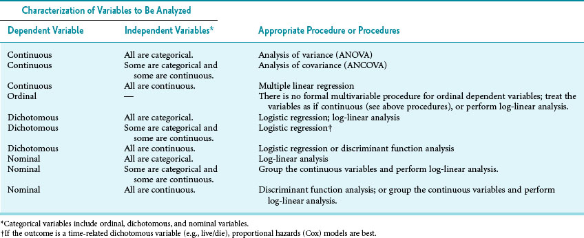
Numerous procedures for multivariable analysis are based on the general linear model. These include methods with such imposing designations as analysis of variance (ANOVA), analysis of covariance (ANCOVA), multiple linear regression, multiple logistic regression, the log-linear model, and discriminant function analysis. As discussed subsequently and outlined in Table 13-1, the choice of which procedure to use depends primarily on whether the dependent and independent variables are continuous, dichotomous, nominal, or ordinal. Knowing that the procedures listed in Table 13-1 are all variations of the same theme (the general linear model) helps to make them less confusing. Detailing these methods is beyond the scope of this text but readily available both online* and in print.4


Stay updated, free articles. Join our Telegram channel

Aug 27, 2016 | Posted by in PUBLIC HEALTH AND EPIDEMIOLOGY | Comments Off on Multivariable Analysis

Full access? Get Clinical Tree

Get Clinical Tree app for offline access