1 Develop Null Hypothesis and Alternative Hypothesis

The first step consists of stating the null hypothesis and the alternative hypothesis. The null hypothesis states that there is no real (true) difference between the means (or proportions) of the groups being compared (or that there is no real association between two continuous variables). For example, the null hypothesis for the data presented in Table 9-2 is that, based on the observed data, there is no true difference between the percentage of men and the percentage of women who had previously had their serum cholesterol levels checked.

It may seem strange to begin the process by asserting that something is not true, but it is much easier to disprove an assertion than to prove that something is true. If the data are not consistent with a hypothesis, the hypothesis should be rejected and the alternative hypothesis accepted instead. Because the null hypothesis stated there was no difference between means, and that was rejected, the alternative hypothesis states that there must be a true difference between the groups being compared. (If the data are consistent with a hypothesis, this still does not prove the hypothesis, because other hypotheses may fit the data equally well or better.)

Consider a hypothetical clinical trial of a drug designed to reduce high blood pressure among patients with essential hypertension (hypertension occurring without an organic cause yet known, such as hyperthyroidism or renal artery stenosis). One group of patients would receive the experimental drug, and the other group (the control group) would receive a placebo. The null hypothesis might be that, after the intervention, the average change in blood pressure in the treatment group will not differ from the average change in blood pressure in the control group. If a test of significance (e.g., t-test on average change in systolic blood pressure) forces rejection of the null hypothesis, the alternative hypothesis—that there was a true difference in the average change in blood pressure between the two groups—would be accepted. As discussed later, there is a statistical distinction between hypothesizing that a drug will or will not change blood pressure, versus hypothesizing whether a drug will or will not lower blood pressure. The former does not specify a directional inclination a priori (before the fact) and suggests a “two-tailed” hypothesis test. The latter does suggest a directional inclination and suggests a “one-tailed” test.

2 Establish Alpha Level

Second, before doing any calculations to test the null hypothesis, the investigator must establish a criterion called the alpha level, which is the highest risk of making a false-positive error that the investigator is willing to accept. By custom, the level of alpha is usually set at p = 0.05. This says that the investigator is willing to run a 5% risk (but no more) of being in error when rejecting the null hypothesis and asserting that the treatment and control groups truly differ. In choosing an arbitrary alpha level, the investigator inserts value judgment into the process. Because that is done before the data are collected, however, it avoids the post hoc (after the fact) bias of adjusting the alpha level to make the data show statistical significance after the investigator has looked at the data.

An everyday analogy may help to simplify the logic of the alpha level and the process of significance testing. Suppose that a couple were given instructions to buy a silver bracelet for a friend during a trip, if one could be bought for $50 or less. Any more would be too high a price to pay. Alpha is similar to the price limit in the analogy. When alpha has been set (e.g., at p ≤0.05, analogous to ≤$50 in the illustration), an investigator would buy the alternative hypothesis of a true difference if, but only if, the cost (in terms of the probability of being wrong in rejecting the null hypothesis) were no greater than 1 in 20 (0.05). The alpha is analogous to the amount an investigator is willing to pay, in terms of the risk of being wrong, if he or she rejects the null hypothesis and accepts the alternative hypothesis.

3 Perform Test of Statistical Significance

When the alpha level is established, the next step is to obtain the p value for the data. To do this, the investigator must perform a suitable statistical test of significance on appropriately collected data, such as data obtained from a randomized controlled trial (RCT). This chapter and Chapter 11 focus on some suitable tests. The p value obtained by a statistical test (e.g., t-test, described later) gives the probability of obtaining the observed result by chance rather than as a result of a true effect. When the probability of an outcome being caused by chance is sufficiently remote, the null hypothesis is rejected. The p value states specifically just how remote that probability is.

Usually, if the observed p value in a study is ≤0.05, members of the scientific community who read about an investigation accept the difference as being real. Although setting alpha at ≤0.05 is arbitrary, this level has become so customary that it is wise to provide explanations for choosing another alpha level or for choosing not to perform tests of significance at all, which may be the best approach in some descriptive studies. Similarly, two-tailed tests of hypothesis, which require a more extreme result to reject the null hypothesis than do one-tailed tests, are the norm; a one-tailed test should be well justified. When the directional effect of a given intervention (e.g., it can be neutral or beneficial, but is certain not to be harmful) is known with confidence, a one-tailed test can be justified (see later discussion).

4 Compare p Value Obtained with Alpha

After the p value is obtained, it is compared with the alpha level previously chosen.

5 Reject or Fail to Reject Null Hypothesis

If the p value is found to be greater than the alpha level, the investigator fails to reject the null hypothesis. Failing to reject the null hypothesis is not the same as accepting the null hypothesis as true. Rather, it is similar to a jury’s finding that the evidence did not prove guilt (or in the example here, did not prove the difference) beyond a reasonable doubt. In the United States a court trial is not designed to prove innocence. The defendant’s innocence is assumed and must be disproved beyond a reasonable doubt. Similarly, in statistics, a lack of difference is assumed, and it is up to the statistical analysis to show that the null hypothesis is unlikely to be true. The rationale for using this approach in medical research is similar to the rationale in the courts. Although the courts are able to convict the guilty, the goal of exonerating the innocent is an even higher priority. In medicine, confirming the benefit of a new treatment is important, but avoiding the use of ineffective therapies is an even higher priority (first, do no harm).

If the p value is found to be less than or equal to the alpha level, the next step is to reject the null hypothesis and to accept the alternative hypothesis, that is, the hypothesis that there is in fact a real difference or association. Although it may seem awkward, this process is now standard in medical science and has yielded considerable scientific benefits.

1 Standard Deviation and Standard Error

Chapter 9 focused on individual observations and the extent to which they differed from the mean. One assertion was that a normal (gaussian) distribution could be completely described by its mean and standard deviation. Figure 9-6 showed that, for a truly normal distribution, 68% of observations fall within the range described as the mean ± 1 standard deviation, 95.4% fall within the range of the mean ± 2 standard deviations, and 95% fall within the range of the mean ± 1.96 standard deviations. This information is useful in describing individual observations (raw data), but it is not directly useful when comparing means or proportions.

Because most research is done on samples, rather than on complete populations, we need to have some idea of how close the mean of our study sample is likely to come to the real-world mean (i.e., mean in underlying population from whom the sample came). If we took 100 samples (such as might be done in multicenter trials), the means in our samples would differ from each other, but they would cluster around the true mean. We could plot the sample means just as we could plot individual observations, and if we did so, these means would show their own distribution. This distribution of means is also a normal (gaussian) distribution, with its own mean and standard deviation. The standard deviation of the distribution of means is called something different, the standard error, because it helps us to estimate the probable error of our sample mean’s estimate of the true population mean. The standard error is an unbiased estimate of the standard error in the entire population from whom the sample was taken. (Technically, the variance is an unbiased estimator of the population variance, and the standard deviation, although not quite unbiased, is close enough to being unbiased that it works well.)

The standard error is a parameter that enables the investigator to do two things that are central to the function of statistics. One is to estimate the probable amount of error around a quantitative assertion (called “confidence limits”). The other is to perform tests of statistical significance. If the standard deviation and sample size of one research sample are known, the standard error can be estimated.

The data shown in Table 10-1 can be used to explore the concept of standard error. The table lists the systolic and diastolic blood pressures of 26 young, healthy, adult subjects. To determine the range of expected variation in the estimate of the mean blood pressure obtained from the 26 subjects, the investigator would need an unbiased estimate of the variation in the underlying population. How can this be done with only one small sample?

Table 10-1 Systolic and Diastolic Blood Pressure Values of 26 Young, Healthy, Adult Participants

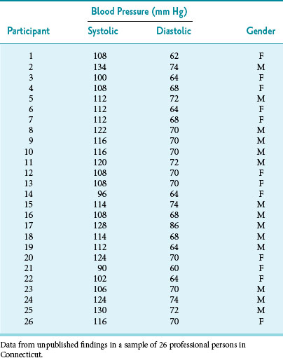
Although the proof is not shown here, an unbiased estimate of the standard error can be obtained from the standard deviation of a single research sample if the standard deviation was originally calculated using the degrees of freedom (N − 1) in the denominator (see Chapter 9). The formula for converting this standard deviation (SD) to a standard error (SE) is as follows:

The larger the sample size (N), the smaller is the standard error, and the better the estimate of the population mean. At any given point on the x-axis, the height of the bell-shaped curve for the distribution of the sample means represents the relative probability that a single sample mean would have that value. Most of the time, the sample mean would be near the true mean, which would be estimated closely by the mean of the means. Less often, it would be farther away from the average of the sample means.

In the medical literature, means are often reported either as the mean ± 1 SD or as the mean ± 1 SE. Reported data must be examined carefully to determine whether the SD or the SE is shown. Either is acceptable in theory because an SD can be converted to an SE, and vice versa, if the sample size is known. Many journals have a policy, however, stating whether the SD or SE must be reported. The sample size should always be shown.

2 Confidence Intervals

The SD shows the variability of individual observations, whereas the SE shows the variability of means. The mean ± 1.96 SD estimates the range in which 95% of individual observations would be expected to fall, whereas the mean ± 1.96 SE estimates the range in which 95% of the means of repeated samples of the same size would be expected to fall. If the value for the mean ± 1.96 SE is known, it can be used to calculate the 95% confidence interval, which is the range of values in which the investigator can be 95% confident that the true mean of the underlying population falls. Other confidence intervals, such as the 99% confidence interval, also can be determined easily. Box 10-2 shows the calculation of the SE and the 95% confidence interval for the systolic blood pressure data in Table 10-1.