A variety of statistical tests can be used to analyze the relationship between two or more variables. Similar to Chapter 10, this chapter focuses on bivariate analysis, which is the analysis of the relationship between one independent (possibly causal) variable and one dependent (outcome) variable. Chapter 13 focuses on multivariable analysis, or the analysis of the relationship of more than one independent variable to a single dependent variable. (The term multivariate technically refers to analysis of multiple independent and multiple dependent variables, although it is often used interchangeably with multivariable). Statistical tests should be chosen only after the types of clinical data to be analyzed and the basic research design have been established. Steps in developing a research protocol include posing a good question; establishing a research hypothesis; establishing suitable measures; and deciding on the study design. The selection of measures in turn indicates the appropriate methods of statistical analysis. In general, the analytic approach should begin with a study of the individual variables, including their distributions and outliers, and a search for errors. Then bivariate analysis can be done to test hypotheses and probe for relationships. Only after these procedures have been done, and if there is more than one independent variable to consider, should multivariable analysis be conducted.

I Choosing an Appropriate Statistical Test

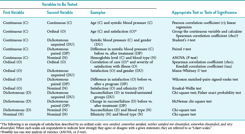
Among the factors involved in choosing an appropriate statistical test are the goals and research design of the study and the type of data being collected. Statistical testing is not required when the results of interest are purely descriptive, such as percentages, sensitivity, or specificity. Statistical testing is required whenever the quantitative difference in a measure between groups, or a change in a measure over time, is of interest. A contrast or change in a measure may be caused by random factors or a meaningful association; statistical testing is intended to make this distinction.

Table 11-1 shows the numerous tests of statistical significance that are available for bivariate (two-variable) analysis. The types of variables and the research design set the limits to statistical analysis and determine which test or tests are appropriate. The four types of variables are continuous data (e.g., levels of glucose in blood samples), ordinal data (e.g., rankings of very satisfied, satisfied, and unsatisfied), dichotomous data (e.g., alive vs. dead), and nominal data (e.g., ethnic group). An investigator must understand the types of variables and how the type of variable influences the choice of statistical tests, just as a painter must understand types of media (e.g., oils, tempera, watercolors) and how the different media influence the appropriate brushes and techniques to be used.

Table 11-1 Choice of Appropriate Statistical Significance Test in Bivariate Analysis (Analysis of One Independent Variable and One Dependent Variable)

The type of research design also is important when choosing a form of statistical analysis. If the research design involves before-and-after comparisons in the same study participants, or involves comparisons of matched pairs of study participants, a paired test of statistical significance (e.g., the paired t-test if one variable is continuous and one dichotomous) would be appropriate. If the sampling procedure in a study is not random, statistical tests that assume random sampling, such as most of the parametric tests, may not be valid.

II Making Inferences (Parametric Analysis) From Continuous Data

Studies often involve one variable that is continuous (e.g., blood pressure) and another variable that is not (e.g., treatment group, which is dichotomous). As shown in Table 11-1, a t-test is appropriate for analyzing these data. A one-way analysis of variance (ANOVA) is appropriate for analyzing the relationship between one continuous variable and one nominal variable. Chapter 10 discusses the use of Student’s and paired t-tests in detail and introduces the concept of ANOVA (see Variation between Groups versus Variation within Groups).

If a study involves two continuous variables, such as systolic blood pressure and diastolic blood pressure, the following questions may be answered:

1. Is there a real relationship between the variables or not?

2. If there is a real relationship, is it a positive or negative linear relationship (a straight-line relationship), or is it more complex?

3. If there is a linear relationship, how strongly linear is it—do the data points almost lie along a straight line?

4. Is the relationship likely to be true and not just a chance relationship?

5. Can the findings be generalized to other populations?

The best way to begin to answer these questions is to plot the continuous data on a joint distribution graph for visual inspection and then to perform correlation analysis and simple linear regression analysis.

The distribution of continuous variables can usually be characterized in terms of the mean and standard deviation. These are referred to as parameters, and data that can be characterized by these parameters can generally be analyzed by methods that rely on them. All such methods of analysis are referred to as parametric, in contrast to nonparametric methods, for which assumptions about the mean and standard deviation cannot be made and are not required. Parametric methods are applicable when the data being analyzed may be assumed to approximate a normal distribution.

A Joint Distribution Graph

The raw data concerning the systolic and diastolic blood pressures of 26 young, healthy, adult participants were introduced in Chapter 10 and listed in Table 10-1. These same data can be plotted on a joint distribution graph, as shown in Figure 11-1. The data lie generally along a straight line, going from the lower left to the upper right on the graph, and all the observations except one are fairly close to the line.

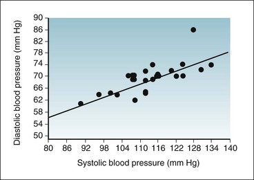
Figure 11-1 Joint distribution graph of systolic (x-axis) and diastolic (y-axis) blood pressure values of 26 young, healthy, adult participants.
The raw data for these participants are listed in Table 10-1. The correlation between the two variables is strong and is positive.

As indicated in Figure 11-2, the correlation between two variables, labeled x and y, can range from nonexistent to strong. If the value of y increases as x increases, the correlation is positive; if y decreases as x increases, the correlation is negative. It appears from the graph in Figure 11-1 that the correlation between diastolic and systolic blood pressure is strong and positive. Based on Figure 11-1, the answer to the first question posed previously is that there is a real relationship between diastolic and systolic blood pressure. The answer to the second question is that the relationship is positive and is almost linear. The graph does not provide quantitative information about how strong the association is (although it looks strong to the eye), and the graph does not reveal the probability that such a relationship could have occurred by chance. To answer these questions more precisely, it is necessary to use the techniques of correlation and simple linear regression. Neither the graph nor these statistical techniques can answer the question of how general the findings are to other populations, however, which depends on research design, especially the method of sampling.

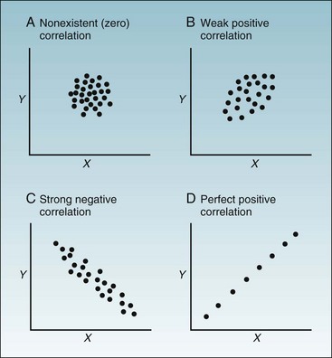
Figure 11-2 Four possible patterns in joint distribution graphs.
As seen in examples A to D, the correlation between two continuous variables, labeled X and Y, can range from nonexistent to perfect. If the value of y increases as x increases, the correlation is positive. If y decreases as x increases, the correlation is negative.

B Pearson Correlation Coefficient

Even without plotting the observations for two continuous variables on a graph, the strength of their linear relationship can be determined by calculating the Pearson product-moment correlation coefficient. This coefficient is given the symbol r, referred to as the r value, which varies from −1 to +1, going through 0. A finding of −1 indicates that the two variables have a perfect negative linear relationship, +1 indicates that they have a perfect positive linear relationship, and 0 indicates that the two variables are totally independent of each other. The r value is rarely found to be −1 or +1, but frequently there is an imperfect correlation between the two variables, resulting in r values between 0 and 1 or between 0 and −1. Because the Pearson correlation coefficient is strongly influenced by extreme values, the value of r can be trusted only when the distribution of each of the two variables to be correlated is approximately normal (i.e., without severe skewness or extreme outlier values).

The formula for the correlation coefficient r is shown here. The numerator is the sum of the covariances. The covariance is the product of the deviation of an observation from the mean of the x variable multiplied by the same observation’s deviation from the mean of the y variable. (When marked on a graph, this usually gives a rectangular area, in contrast to the sum of squares, which are squares of the deviations from the mean.) The denominator of r is the square root of the sum of the squared deviations from the mean of the x variable multiplied by the sum of the squared deviations from the mean of the y variable:

Using statistical computer programs, investigators can determine whether the value of r is greater than would be expected by chance alone (i.e., whether the two variables are statistically associated). Most statistical programs provide the p value along with the correlation coefficient, but the p value of the correlation coefficient can be calculated easily. Its associated t can be calculated from the following formula, and the p value can be determined from a table of t (see Appendix, Table C)¹:

As with every test of significance, for any given level of strength of association, the larger the sample size, the more likely it is to be statistically significant. A weak correlation in a large sample might be statistically significant, despite that it was not etiologically or clinically important (see later and Box 11-5). The converse may also be true; a result that is statistically weak still may be of public health and clinical importance if it pertains to a large portion of the population.

There is no perfect statistical way to estimate clinical importance, but with continuous variables, a valuable concept is the strength of the association, measured by the square of the correlation coefficient, or r². The r² value is the proportion of variation in y explained by x (or vice versa). It is an important parameter in advanced statistics. Looking at the strength of association is analogous to looking at the size and clinical importance of an observed difference, as discussed in Chapter 10.

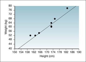
For purposes of showing the calculation of r and r², a small set of data is introduced in Box 11-1. The data, consisting of the observed heights (variable x) and weights (variable y) of eight participants, are presented first in tabular form and then in graph form. When r is calculated, the result is 0.96, which indicates a strong positive linear relationship and provides quantitative information to confirm what is visually apparent in the graph. Given that r is 0.96, r² is (0.96),² or 0.92. A 0.92 strength of association means that 92% of the variation in weight is explained by height. The remaining 8% of the variation in this sample is presumed to be caused by factors other than height.

Box 11-1 Analysis of Relationship between Height and Weight (Two Continuous Variables) in Eight Study Participants

Part 1 Tabular and Graphic Representation of the Data

Part 2 Calculation of Moments

Note: Moments are various descriptors of a distribution, including the number of observations, the sum of their values, the mean, the variance, the standard deviation, and tests of normality.

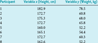
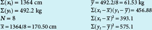
Part 3 Calculation of Pearson Correlation Coefficient (r) and Strength of Association of Variables (r²)

Interpretation: The two variables are highly correlated. The association between the two variables is strong and positive with 92% of variation in weight (y) explained by variation in height (x).

Part 4 Calculation of the Slope (b) for a Regression of Weight (y) on Height (x)

Interpretation: There is a 1.16-kg increase in weight (y) for each 1-cm increase in height (x). The y-intercept, which indicates the value of x when y is 0, is not meaningful in the case of these two variables, and it is not calculated here.

Data from unpublished findings in a sample of eight professional persons in Connecticut.

C Linear Regression Analysis

Linear regression is related to correlation analysis, but it produces two parameters that can be directly related to the data: the slope and the intercept. Linear regression seeks to quantify the linear relationship that may exist between an independent variable x and a dependent variable y, whereas correlation analysis seeks to measure the strength of correlation. More specifically, regression specifies how much y would be expected to change (and in what direction) for a unit change in x. Correlation analysis indicates whether y changes proportionately with changes in x.

The formula for a straight line, as expressed in statistics, is y = a + bx (see Chapter 10). The y is the value of an observation on the y-axis; x is the value of the same observation on the x-axis; a is the regression constant (value of y when value of x is 0); and b is the slope (change in value of y for a unit change in value of x). Linear regression is used to estimate two parameters: the slope of the line (b) and the y-intercept (a). Most fundamental is the slope, which determines the impact of variable x on y. The slope can tell how much weight is expected to increase, on the average, for each additional centimeter of height.

When the usual statistical notation is used for a regression of y on x, the formulas for the slope (b) and y-intercept (a) are as follows:

Box 11-1 shows the calculation of the slope (b) for the observed heights and weights of eight participants. The graph in Box 11-1 shows the linear relationship between the height and weight data, with the regression line inserted. In these eight participants, the slope was 1.16, meaning that there was an average increase of 1.16 kg of weight for every 1-cm increase in height.

Linear regression analysis enables investigators to predict the value of y from the values that x takes. The formula for linear regression is a form of statistical modeling, where the adequacy of the model is determined by how closely the value of y can be predicted from the other variable. It is of interest to see how much the systolic blood pressure increases, on the average, for each added year of age. Linear regression is useful in answering routine questions in clinical practice, such as, “How much exercise do I need to do to raise my HDL 10 points, or lose 10 pounds?” Such questions involve the magnitude of change in a given factor, y, for a specific change in behavior, or exposure, x.

Just as it is possible to set confidence intervals around parameters such as means and proportions (see Chapter 10), it is possible to set confidence intervals around the parameters of the regression, the slope, and the intercept, using computations based on linear regression formulas. Most statistical computer programs perform these computations, and moderately advanced statistics books provide the formulas.² Multiple linear regression and other methods involved in the analysis of more than two variables are discussed in Chapter 13.

III Making Inferences (Nonparametric Analysis) From Ordinal Data

Many medical data are ordinal, meaning the observations can be ranked from the lowest value to the highest value, but they are not measured on an exact scale. In some cases, investigators assume that ordinal data meet the criteria for continuous (measurement) data and analyze these variables as though they had been obtained from a measurement scale. If patients’ satisfaction with the care in a given hospital were being studied, the investigators might assume that the conceptual distance between “very satisfied” (e.g., coded as a 3) and “fairly satisfied” (coded as a 2) is equal to the difference between “fairly satisfied” (coded as a 2) and “unsatisfied” (coded as a 1). If the investigators are willing to make these assumptions, the data might be analyzed using the parametric statistical methods discussed here and in Chapter 10, such as t-tests, analysis of variance, and analysis of the Pearson correlation coefficient. This assumption is dubious, however, and seldom appropriate for use in publications.

If the investigator is not willing to assume an ordinal variable can be analyzed as though it were continuous, many bivariate statistical tests for ordinal data can be used ^1,³ (see Table 11-1 and later description). Hand calculation of these tests for ordinal data is extremely tedious and invites errors. No examples are given here, and the use of a computer for these calculations is customary.

Tests specific for ordinal data are nonparametric because they do not require assumptions about the mean and standard deviation of the data, known as parameters, and are not dependent on them.

A Mann-Whitney U Test

The test for ordinal data that is similar to the Student’s t-test is the Mann-Whitney U test. U, similar to t, designates a probability distribution. In the Mann-Whitney test, all the observations in a study of two samples (e.g., experimental and control groups) are ranked numerically from the smallest to the largest, without regard to whether the observations came from the experimental group or from the control group. Next, the observations from the experimental group are identified, the values of the ranks in this sample are summed, and the average rank and the variance of those ranks are determined. The process is repeated for the observations from the control group. If the null hypothesis is true (i.e., if there is no real difference between the two samples), the average ranks of the two samples should be similar. If the average rank of one sample is considerably greater than that of the other sample, the null hypothesis probably can be rejected, but a test of significance is needed to be sure. Because the U-test method is tedious, a t-test can be done instead (considering the ranks as though they were continuous data), and often this yields similar results.¹

The Mann-Whitney U test was applied, for example, in a study comparing lithotripsy to ureteroscopy in the treatment of renal calculi.⁴

B Wilcoxon Matched-Pairs Signed-Ranks Test

The rank-order test that is comparable to the paired t-test is the Wilcoxon matched-pairs signed-ranks test. In this test, all the observations in a study of two samples are ranked numerically from the largest to the smallest, without regard to whether the observations came from the first sample (e.g., pretreatment sample) or from the second sample (e.g., posttreatment sample). After pairs of data are identified (e.g., pretreatment and posttreatment observations are linked), the pretreatment-posttreatment difference in rank is identified for each pair. For example, if for a given pair the pretreatment observation scored 7 ranks higher than the posttreatment observation, the difference would be noted as −7. If in another pair the pretreatment observation scored 5 ranks lower than the posttreatment observation, the difference would be noted as +5. Each pair would be scored in this way. If the null hypothesis were true (i.e., if there were no real difference between the samples), the sum of the positive and negative scores should be close to 0. If the average difference is considerably different from 0, the null hypothesis can be rejected.

The Wilcoxon test, for example, was used to compare knowledge, attitude, and practice measures between groups in an educational program for type 1 diabetes.⁵

C Kruskal-Wallis Test

If the investigators in a study involving continuous data want to compare the means of three or more groups simultaneously, the appropriate test is a one-way analysis of variance (a one-way ANOVA), usually called an F-test. The comparable test for ordinal data is called the Kruskal-Wallis test or the Kruskal-Wallis one-way ANOVA. As in the Mann-Whitney U test, for the Kruskal-Wallis test, all the data are ranked numerically, and the rank values are summed in each of the groups to be compared. The Kruskal-Wallis test seeks to determine if the average ranks from three or more groups differ from one another more than would be expected by chance alone. It is another example of a critical ratio (see Chapter 10), in which the magnitude of the difference is in the numerator, and a measure of the random variability is in the denominator. If the ratio is sufficiently large, the null hypothesis is rejected.

The Kruskal-Wallis test was used, for example, in an analysis of the effects of electronic medical record systems on the quality of documentation in primary care.⁶

D Spearman and Kendall Correlation Coefficients

When relating two continuous variables to each other, investigators can use regression analysis or correlation analysis. For ordinal variables, there is no test comparable to regression because it is difficult to see how a slope could be measured without an underlying measurement scale. For ordinal data, however, several tests are comparable to correlation, the two most common of which are briefly defined here. The first is the Spearman rank correlation coefficient, whose symbol is the Greek letter rho; it is similar to r. The second is the Kendall rank correlation coefficient, which is symbolized by the Greek letter tau. (Actually, tau comes in three forms, depending on whether the test makes use of or ignores ties in the data, and whether the table being analyzed is symmetric or not. Most tables to which tau is applied are symmetric and may have ties in the data—for this, Kendall’s tau-b is used.) The tests for rho and tau usually give similar results, but the rho is usually used in the medical literature, perhaps because of its conceptual similarity to the Pearson r. The tau may give better results with small sample sizes.

The Spearman rank test was used, for example, in a validation study of a tool to address the preservation, for example, dignity at end of life.⁷

E Sign Test

Sometimes an experimental intervention produces positive results on most of many different measurements, but few, if any, of the individual outcome variables show a difference that is statistically significant. In this case, the sign test can be extremely helpful to compare the results in the experimental group with those in the control group. If the null hypothesis is true (i.e., there is no real difference between the groups), by chance, the experimental group should perform better on about half the measurements, and the control group should perform better on about half.

The only data needed for the sign test are the records of whether, on the average, the experimental participants or the control participants scored “better” on each outcome variable (by what amount is not important). If the average score for a given variable is better in the experimental group, the result is recorded as a plus sign (+); if the average score for that variable is better in the control group, the result is recorded as a minus sign (−); and if the average score in the two groups is exactly the same, no result is recorded, and the variable is omitted from the analysis. For the sign test, “better” can be determined from a continuous variable, ordinal variable, dichotomous variable, clinical score, or component of a score. Because under the null hypothesis the expected proportion of plus signs is 0.5 and of minus signs is 0.5, the test compares the observed proportion of successes with the expected value of 0.5.

The sign test was employed, for example, in a study of the effect of an electronic classroom communication device on medical student examination scores.⁸

IV Making Inferences (Nonparametric Analysis) From Dichotomous and Nominal Data

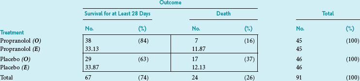
As indicated in Table 11-1, the chi-square test, Fisher exact probability test, and McNemar chi-square test can be used in the analysis of dichotomous data, although they use different statistical theory. Usually, the data are first arranged in a 2 × 2 table, and the goal is to test the null hypothesis that the variables are independent.

A 2 × 2 Contingency Table

Data arranged as in Box 11-2 form what is known as a contingency table because it is used to determine whether the distribution of one variable is conditionally dependent (contingent) on the other variable. More specifically, Box 11-2 provides an example of a 2 × 2 contingency table, meaning that it has two cells in each direction. In this case, the table shows the data for a study of 91 patients who had a myocardial infarction.⁹ One variable is treatment (propranolol vs. a placebo), and the other is outcome (survival for at least 28 days vs. death within 28 days).

Box 11-2 Chi-Square Analysis of Relationship between Treatment and Outcome (Two Nonparametric Variables, Unpaired) in 91 Participants

Tags: Jekels Epidemiology Biostatistics and Preventive Medicine

Aug 27, 2016 | Posted by admin in PUBLIC HEALTH AND EPIDEMIOLOGY | Comments Off

Basicmedical Key

Fastest Basicmedical Insight Engine

Bivariate Analysis