Model quantum systems
There are two different aspects of this chapter to emphasize. One is that it provides practice in the application of quantum mechanical methods to model physical systems. We learn how to apply the mathematics of quantum mechanics to the solution of physical problems. We learn how to interpret quantum mechanical results and behavior. But more than that, the systems presented here also represent the first-order approximations to the behavior of a wide variety of actual physical systems. They are our first attempts at developing the language that will allow us to describe quantum mechanical phenomena. Applying perturbations to these model systems quite frequently allows us to model and understand the behavior of real systems with terms familiar to us from the classical world.
We have already treated one model system – the free particle – in detail in Chapter 20. We also encountered the particle in a box and the harmonic oscillator in Chapter 20. The model atomic system, the H atom, is treated in Chapter 22. For the H atom problem, we will see how we can exploit similarities in the physics of models of rotational motion to solving the energy level structure of atoms.
21.1 Particle in a box
21.1.1 One-dimensional box
Consider a particle confined to a box where the potential energy is V(x) inside the box and goes to infinity outside the box. The width of the box is given the value a. The particle cannot penetrate the walls of the box because its potential energy is infinite there. If the walls are not infinitely tall, some penetration of the walls will occur. This is the origin of tunneling, which we will investigate below. This particle in a box problem is also known as the infinite square well.
We begin by writing the Hamiltonian,

where V(x) = 0 for 0 ≤ x ≤ a and V(x) = ∞ elsewhere. This potential confines the particle to be inside the box, which forces the wavefunction to go to zero at the walls and to vanish everywhere outside of the box. In the box the Schrödinger equation is

To solve Eq. (21.2), we try inserting a general trial solution for ψ(x),

We simplify this solution further by considering the boundary conditions,

That the wavefunction goes to zero at the walls is clear in Fig. 21.1. Thus, at x = 0,

which requires that B = 0. At x = a,

this means that ka = nπ thus k = nπ/a, where n is an integer.

Figure 21.1 Potential energy diagram of the particle in a one-dimensional box with infinitely high walls and box length a. Classically all values of energy are allowed, but quantum mechanically only quantized energy levels are allowed. The energy of these levels increases with n2, where n is a quantum number that defines the state. The first six allowed levels are included. The wavefunction of the n = 5 level is also shown. The wavefunction goes to zero at the walls of the box and is identically zero outside of the box.
We use this infinite set of wavefunctions to solve the Schrödinger equation, which reveals a formula for the energies of the levels associated with each wavefunction.

This has the solution

The allowed energies are not continuous. Only certain values are allowed. That is, now that the particle is confined to the box rather than translating freely, the energy is quantized.
To find the complete form of the wavefunction, we must normalize our trial solution. Normalization ensures that the probability of finding the particle in the box is exactly one.


The trial solution reduces to

and the complete set of normalized wavefunction is  for 0 ≤ x ≤ a and ψn(x) = 0 otherwise. Note that this is a case where the derivative of the wavefunction is not continuous in two spots, namely, at x = 0 and x = a. Nonetheless, the wavefunction is continuous at these points and the wavefunction is a good wavefunction for describing the particle in the box. There is no wavefunction outside the box so that there is nothing to describe there.
Notice a few characteristics of this solution:
- Confinement along one coordinate in the problem leads to one quantum number (n) being required to define the energy.
- There are an infinite number of wavefunctions, the quantum number n ranges from 1 to ∞.
- Each wavefunction has a different energy and each energy corresponds to only one wavefunction. This means that the eigenstates are non-degenerate.
- The lowest energy state (the ground state) is not at E = 0; instead, it has a finite zero point energy (ZPE) associated with it.
- There is zero probability of finding the particle at the nodes.
- Higher energy corresponds to a greater number of nodes. This is true for any potential.
- The wavefunction changes sign at nodes.
- Wavefunctions are symmetrical about the middle of the box and alternate being even and odd with respect to the center of the well. This is true for any symmetric potential.
- The overlap between the different wavefunctions is zero; they are orthogonal.
Orthogonality means that the wavefunctions corresponding to different quantum numbers (i.e., n = 1, 2, 3…) do not mix with each other. Mathematically, orthogonality is expressed by the following equation:1

21.1.1.1 Example
Find the wavelength of light emitted when a 1 × 10–27 g particle in a 3-Å one-dimensional box goes from the n = 2 to the n = 1 level.
The wavelength λ can be found from the frequency ν. The quantity hν is the energy of the emitted photon and equals the energy difference between the two levels involved in the transition

Then, from λ = c/ν,
This wavelength is in the UV.
21.1.1.2 Directed practice
Confirm that the wavefunction in Eq. (21.11) satisfies the Schrödinger equation inside of the box.
21.1.2 Three-dimensional box
Perhaps only a string theorist could consider a one-dimensional box a box. Boxes in the macroscopic world correspond to three-dimensional boxes. How does the problem change should it be extended to three dimensions? Let’s first assume that our box has edges placed along the Cartesian coordinate axes x, y, and z with edge length Lx, Ly, and Lz. The origin is placed at one of the vertices of this box. The potential is zero inside the box and infinite outside of it, such that

Our particle has mass m. Its kinetic energy is equal to the total energy of the system; thus the Hamiltonian is

and the Schrödinger equation is

where ∇2 is the Laplacian operator introduced in the last chapter. To solve this problem we can again introduce separation of variables. The Hamiltonian contains no cross-terms, that is, no terms containing x and y or any other combination of coordinates. Thus, it can be written as the sum of three terms, each involving only one coordinate,

where

with ξ = x, y or z as appropriate.
Each term in the Hamiltonian only acts on one coordinate. We found that when we applied separation of variables to the time-dependent Schrödinger equation, we obtained a product wavefunction with one term for each set of separable variables (space and time in that case). This suggests that our wavefunction for the three-dimensional box should also be a product wavefunction of the form

The solution of the Schrödinger equation for any one of the component terms in the Hamiltonian is of exactly the same form as the solution of the one-dimensional problem in the previous section. For example,

Furthermore, since a component term only acts on one coordinate, the other coordinates can be treated as constants for that operator. For example,

The energies and wavefunctions for the y– and z-components must have the same behavior. Substituting this into the Schrödinger equation, we find that the total energy must simply be the sum of the x-, y– and z-contributions

21.1.2.1 Directed practice
Substitute into the Schrödinger equation and prove that the energy of the three-dimensional box is equal to the sum of the x, y and z energy components.
If our particle were confined to a surface, the box would be two-dimensional. The separation of variables treatment used above would also apply. This argument can be generalized to an arbitrary number of dimensions. This also allows us to formulate a general principle
When the Hamiltonian can be written as the sum of terms, each of which depends only on a set of coordinates unique to that term, the corresponding wavefunction can be written as the product of component wavefunctions, each of which depends only on the corresponding set of coordinates.
Since each contribution in Eq. (21.21) is of the form Eξ, n = n2ξh2/8mL2ξ, the total energy of the three-dimensional particle in a box is

Three independent integers now specify each level. Each starts at nξ = 1; thus, there is now a zeropoint energy associated with each coordinate. Specification of three independent integers also introduces the possibility of degeneracy of levels, that is, more than one state existing at the same energy. If the three lengths are all different, this degeneracy would be accidental. If, on the other hand, the box is cubic and L = Lx = Ly = Lz, then degeneracy will occur whenever the sum of the squares of the nξ values is equal. Thus, the state defined by (nx, ny, nz) = (1, 2, 3) is degenerate to the other five states defined by the permutations of 1, 2, and 3. In addition 12 + 12 + 52 = 27 just as 32 + 32 + 32 = 27; therefore, these states as well as the states represented by permutations of 1, 1, and 5 are all degenerate.
21.1.3 Quantum confinement and the correspondence principle
A particle in a cubic box of edge length L has energy levels given by

For spherical confinement instead of cubic in which the particles are confined to executing circular orbits on the surface of a sphere with radius r, the energy levels are given by

Thus, the spacing between successive energy levels is given by

You will see below that this corresponds to a model of rotational motion and the angular dependence of electrons trapped in the potential of a nucleus; hence, the switch to the quantum number l.
The form of the equations changes based on the geometry. If the box were rod-like or ellipsoidal, the equations would be slightly different. However, notice the similarities: (i) the energy level spacing is inversely proportional to length squared; (ii) it is also inversely proportional to the mass; and (iii) in the limit of large quantum numbers, the spacing between successive energy levels becomes negligible.
The emergence of significant quantum mechanical behavior with decreasing size is known as quantum confinement. More precisely, as the de Broglie wavelength of a particle approaches the size of the container formed by the potential that confines it, the more important quantum effects become. Quantum confinement is one of the fundamental phenomena underpinning nanoscience and nanotechnology.
In solid-state systems, an electron excited across a band gap to the conduction band can interact with the hole it left behind in the valence band to form a collective excitation (quasi-particle) known as an exciton. An exciton is a pseudo-hydrogenic system that has a characteristic exciton Bohr radius

where μ is the reduced mass of the exciton. For reasons related to the band structure of the material – that is, the potential that binds the electrons – the effective mass of the electron and the hole do not equal the mass of a free electron. The exciton radius of Si is 4.9 nm, that of GaAs is 14 nm, and that of InSb is 69 nm. When the size of a semiconductor nanoparticle approaches and then becomes less than the exciton radius, quantum confinement effects set in. As demonstrated by Leigh Canham,2 when silicon nanoparticles become smaller than about 5 nm, the properties of the nanoscale Si particles change dramatically: the particles become visibly luminescent (as shown in Fig. 21.3) and the wavelength of the luminescence shifts to the blue (higher energy) as the size of the particles become smaller. Theoretical calculations made by Birgitta Whaley’s group3 show that the increase of the band gap resulting from the shift of the conduction band upward and the valence band downward can explain the shift of the photoluminescence with decreasing nanocrystal size. The size dependence is much like that expected from the application of Eq. (21.24). Other properties, such as the absorption spectrum, phonon spectrum (how the solid vibrates), thermal and electrical conductivity, and chemical reactivity also become size-dependent. Such quantum-confined nanoparticles are known as quantum dots.

Figure 21.2 (a) Wavefunctions and (b) the square of the wavefunction for the particle in a box from n = 1 to n = 8. Note how the symmetry about the center of the box at x/a = 0.5 alternates from even to odd as n increases. The wavefunction changes sign about either side of a node. The number of extrema equals n and the number of nodes is n – 1.

Figure 21.3 Photoluminescence emitted from nanocrystalline porous silicon under excitation with ultraviolet light. The crystal in the upper right corner is bulk crystalline Si. It does not luminesce. The other crystals are covered with layers of nanocrystalline porous silicon produced under different conditions to achieve different crystallite sizes. The luminescence spectrum of the freshly produced nanocrystals shifts to the blue (from red to yellow to green) with smaller size.4
A quantum dot is a system that is confined in three dimensions. Therefore, it has zero degrees of freedom and a quantum dot is a zero-dimensional (OD) system. Quantum dots have also been called artificial atoms because they have energy level structures that are analogous to those of atoms. They have discrete energy levels with sharp energies. A quantum wire is confined in two dimensions and represents a one-dimensional (1D) system. A quantum well is confined in one dimension and is a 2D system. One-, two-, and three-dimensional structures exhibit energy bands rather than discrete states.
The antithesis of quantum confinement is Bohr’s correspondence principle.5 When r is large enough the energy levels are spaced continuously. The system evolves toward classical behavior as the system leaves the nanoscale and enters the microscale. In the limit of large radii, large quantum numbers and large masses quantum mechanical behavior converges on classical behavior.
21.2 Quantum tunneling
In classical mechanics a particle with energy E encountering a barrier of height V0 cannot surmount the barrier unless it has sufficient energy to do so, E > V0. But the rules of classical mechanics do not apply to quantum particles. In quantum mechanics, subatomic (and sometimes larger) particles can overcome a barrier even if they do not have sufficient energy to overcome it. This process, shown schematically in Fig. 21.4 is known as quantum mechanical tunneling. Tunneling is involved in the explanation of the radioactivity of atomic nuclei by alpha particle decay. It can contribute to kinetic isotope effects, especially in proton-transfer reactions, including those catalyzed by enzymes. Tunneling is also the basis of the technique known as scanning tunneling microscopy (STM), which allows us to ‘see’ atoms. More accurately, it allows us to image the electronic states of atoms and molecules. Since the electronic states are often (though not always) strongly correlated with the positions of atoms, the contours of these images can reflect the positions of the atomic nuclei at the core of atoms, as shown in Fig. 21.5(b).

Figure 21.4 A particle approaching a barrier of height V0 and width L from the left. The wavefunction decays exponentially inside the barrier and then re-emerges on the right side. Transmission through a barrier, even when the particle energy is less than the classical barrier height, is known as tunneling.

Figure 21.5 (a) Schematic representation of STM. A sharp metal tip is rastered across a surface in the x– and y-directions while held at potential U. Control of the potential allows electrons to tunnel either from the occupied electronic states of the tip into the unoccupied states of the surface, or vice versa. Holding this tunneling current constant by moving the tip up and down in the z direction while scanning in the xy plane, the contours of the surface are mapped with atomic resolution. (b). An STM image of a CoMoS nanocluster that acts as a desulfurization catalyst. Provided by Flemming Besenbacher. Reproduced with permission from Lauritsen, J.V., Vang, R.T., and Besenbacher, F. (2006) Catal. Today, 111, 34; © 2006 Elsevier Science.
Figure 21.4 illustrates an important characteristic of the wavefunction:
The wavefunction and it first derivative must be continuous and finite.
This may seem like formal mathematical details. However, if the wavefunction changed discontinuously at the barrier wall, the first derivative would be infinite. From the Schrödinger equation we know that an infinite second derivative translates into an infinite energy. This cannot be, so the wavefunction approaching the barrier from the left must be equal to the wavefunction approaching the barrier from the right at the point where they meet. In the coordinate system of Fig. 21.4, this point is x = 0, thus

Similarly,

The two analogous boundary conditions apply on the right side of the barrier as the particle exits (if it can exit) the barrier at x = L.
When the free particle meets the barrier as it travels from left to right, a portion of the wave is reflected and a portion enters the barrier. The wavefunction on the left is

As before, when we treated free particle motion in Section 20.6, the relationship between energy and wavevector is

On the right side of the barrier, the particle only translates to the right and the wavefunction is

The constant A is the incident amplitude, B is the reflected amplitude, and F is the transmitted amplitude. The transmission coefficient T is given by the ratio of probability flux

These coefficients are determined by applying the boundary conditions as in Eqs. (21.27) and (21.28).
Tunneling occurs because the wavefunction of the particle is able to penetrate the barrier into what is energetically a classically forbidden region. The transmission probability depends on the energy of the particle E compared to the barrier height V0, the mass of the particle m, as well as the shape and thickness L of the barrier. Tunneling is more important for energies close to the top of the barrier, light particles (muons, electrons and oftentimes even protons) and thin smooth barriers. In particular, tunneling is important when the thickness of the barrier becomes comparable to the de Broglie wavelength of the particle.
Within the classically forbidden region inside the barrier, the wavefunction of the particle decays exponentially

where the decay constant κ is

The transmission coefficient is determined by applying to continuity conditions from Eqs. (21.27) and (21.28) at both x = 0 and x = L, from which we obtain

where Γ is the decay length,

Typical values of κ lie in the range of about 0.8–1.2 Å–1 for many electron transfer events of interest in chemistry. Thus, tunneling usually is effective over a range of a few Å. One such example of this is outer-sphere electron transfer in electrochemistry. Electron transfer occurs when an electron hops from the donor to the acceptor, which are separated by a distance r. There is a Gibbs energy of activation associated with electron transfer Δ‡Gm°. The rate of electron transfer is proportional to the product of the Arrhenius activation term and the exponential distance dependence,

If a sharp metal tip is brought close to a surface, as shown in Fig. 21.5(a), a tunneling current will flow when the wavefunction of an electron in the tip overlaps spatially and energetically with the wavefunction of the surface. Charge transfer always occurs from occupied to unoccupied (or partially occupied) states, and the direction of flow (tip to surface or surface to tip) can be controlled by placing a voltage on the tip relative to the surface. The current that flows is highly sensitive to the distance between the two. It is proportional to the transmission coefficient

This exponential dependence of the tunneling current on the distance L between the tip and the surface is the basis of scanning tunneling microscopy, for which its inventors Gerd Binnig and Heinrich Rohrer were awarded the Nobel Prize in Physics 1986.6
For V0 – E = 4.5 eV, a change from L = 0.2 nm to L = 0.3 nm changes the current by a factor of 8.8. At L = 0.2 nm, changing from the mass of an electron to the mass of a proton decreases the current by 1.2 × 10–79. It is easy to understand why tunneling probe microscopy is exceedingly sensitive to height variations and involves the tunneling of electrons rather than more massive particles.
21.3 Vibrational motion
One of the reasons that the harmonic oscillator is so versatile is that in the vicinity of a local minimum almost any potential is approximately harmonic. This is shown in Fig. 21.6 and can be explained in the following manner. Expand the potential V(r) in a Taylor series about the local minimum located at re,

where V′ is the first derivative with respect to r and V″ the second. The constant is inconsequential because it does not change the force, which is given by the negative of the derivative of the potential

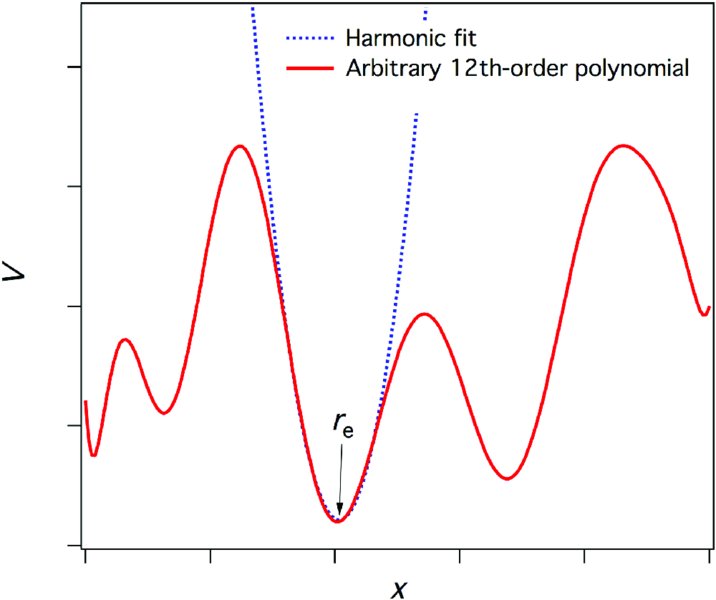
Figure 21.6 The harmonic approximation to a local minimum in an arbitrary potential constructed from a 12th-order polynomial.
At the minimum, the first derivative is zero. Neglecting higher order terms, which should be small as long as the displacement from the minimum, x = r − re, is small, the potential is approximately,

Taking the derivative we obtain,

which is Hooke’s law for harmonic motion of a frictionless spring. The force constant k is then identified as

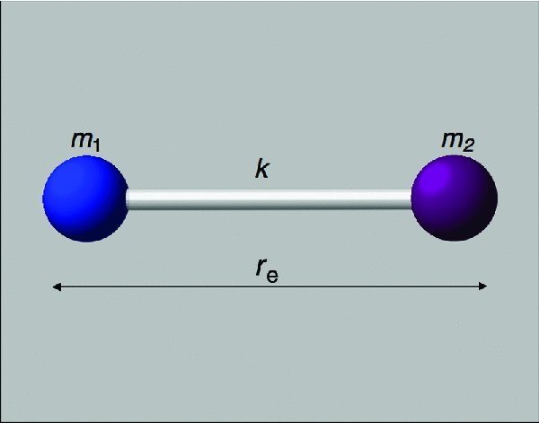
Figure 21.7 A harmonic oscillator with an equilibrium separation re between masses m1 and m2. The coordinate x along the spring axis measures the displacement from this equilibrium value. The masses are connected by a massless spring of force constant k.
The force constant is related to the fundamental vibrational angular frequency of the oscillator by7

Stay updated, free articles. Join our Telegram channel

Full access? Get Clinical Tree


