Introduction to spectroscopy and atomic spectroscopy
Spectroscopy is the study of transitions between energy levels. Commonly, these transitions involve the interaction of photons with atoms or molecules, as we have discussed, for example, in the spectroscopy of the H atom. However, because of wave-particle duality there is also spectroscopy performed with the excitation provided by electrons, which can act as waves to engender many of the same transitions as photons but without the restrictions on changing electron spin. This was the basis of the experiments by Franck and Hertz in which light emission from Hg atoms was excited by electron irradiation. Spectroscopy can also be performed between bound and unbound levels; this is the case in photoelectron spectroscopy. Spectroscopy is the most important method of investigating the world of atoms and molecules, and its importance has increased since the invention of the laser. The applications of lasers in atomic, molecular and chemical physics continue to develop and refine our understanding of chemical processes and the interactions between atoms and molecules.
You are already aware of the fundamentals of spectroscopy. You are already familiar with the role of conservation of energy. Conservation of energy and angular momentum set the rules for spectroscopy. In this chapter we will delve into the ramification of angular momentum in more detail.
23.1 Fundamentals of spectroscopy
23.1.1 Terminology
The first thing to remember about spectroscopy is that it involves matter–wave interactions. Thus, the Planck equation

and the fundamental relationships of the speed of light c, frequency ν, wavenumber  , wavelength λ and angular frequency ω

have to kept in mind. Recall the discussion in Chapter 19 that the frequency of light ν is independent of the medium. However, in accord with Eq. (19.3) the wavelength of light in the medium λ must be reduced from its value in vacuo λ0 such that λ = λ0/n. Correspondingly, the wavenumber is increases by a factor of n. Thus, the relations in Eq. (23.1) hold strictly only in vacuum. Much of the remainder of spectroscopy is respecting the implications of conservation of energy and angular momentum.
How much structure we see in spectroscopy depends on how closely we look – that is, on the resolution and the energy scale at which we probe the molecule. We have already encountered this in the spectroscopy of the electronic states of the H atom. As we are beginning with atomic spectroscopy, we need only concern ourselves with the electronic degree of freedom. Most transitions involving the electronic ground state and the first few excited states in atoms occur either in the visible or ultraviolet portions of the electromagnetic spectrum. The density of electronic states increases dramatically as the atom approaches its first ionization limit. In other words, energy level spacings decrease with increasing principal quantum number n. The energies of transitions between these high-lying energy levels can be found at lower energies in the infrared, or below.
As Z increases, the binding of the K shell electrons rapidly increases. In multi-electron atoms we distinguish between core electrons and valence electrons. Core electrons are little influenced by the chemical environment and are not directly involved in bonding. They lie at very low energies and their ionization energies correspond to the vacuum ultraviolet or X-ray regions. Valence electrons are found in the highest energy normally occupied electronic states. Their ionization energies are lower than those of core electrons. Valence electrons participate in bonding. Because they are strongly linked to bonding, the energetic position of valence electron states shift sensitively in response to the chemical environment around an atom.
The shifts in energy of electronic levels is detected by performing spectroscopy of various sorts. There is a great deal of spectroscopic terminology that you need to familiarize yourself with. A number of conventions surround the use of the words ‘red’ and ‘blue’ and the use of energy scales. It is conventional in many settings to place the origin of wavelength on the left. But the wavelength is inversely proportional to photon energy, which means that the origin of photon energy, frequency and wavenumber is often placed on the right. The red side of the visible spectrum is the long-wavelength/low-energy side. The blue end of the visible spectrum is the short-wavelength/high-energy side. Spectroscopists will often speak of the ‘blue end’ or ‘red end’ of a spectrum or of a ‘blue shift’ or ‘red shift’ of peaks. This terminology is used even when referring to other parts of the electromagnetic spectrum. A blue shift is a shift to higher energy, while a red shift is a shift to lower energy. Thus, we say that the a peak in the X-ray photoemission spectrum of the Ti 2P3/2 level is blue shifted from 453.8 eV in Ti metal to 458.5 eV in TiO2, which means that the peak lies at higher energy in TiO2 than in Ti.
When a photon is absorbed, the atom makes a transition from one energy state to an excited state (a state of higher energy). When a photon is emitted, the atom makes a transition from an excited state to a state of lower energy. The lowest energy state in the atom is the ground state.
There are many types of transitions, excitations, and excitation mechanisms. Here, we deal only with atoms, and the only transitions we are interested in involve moving electrons between different energy levels. Other transitions involving rotation, vibration, nuclear spin, and so forth will be discussed in subsequent chapters.
The Ritz combination principle1 states that each atomic state has an energy, and any two states can combine to give rise to a spectral line in either absorption or emission. The energy difference is equal to the photon energy. While all combinations are in principle possible, selection rules mean that some are forbidden and have very low intensities. The strength of a transition is a measure of how likely the transition is to occur. An ‘allowed’ transition is a strong absorber or emitter of photons. A ‘forbidden’ transition is a weak absorber or emitter. There are different degrees of how forbidden a transition is. Lasers, because of their high intensity, allow us to probe very weak transitions that were once thought to be totally forbidden. Alternatively, we might try to use very long pathlengths and the interaction of light with as many atoms as possible to observe a strongly forbidden transition. Selection rules provide indicators of whether a transition is allowed or forbidden. Later, we will develop specific examples of selection rules and determine why they arise. As we shall see, they are related to the conservation of angular momentum and symmetry. The quantitation of how big peaks are gives us information both on how strong a transition is (through the selection rules) and how many atoms are in a particular state. Therefore, spectroscopy can also be used to determine how atoms are distributed among the available quantum states.
Spectroscopy generally involves some type of energy resolution (energy dispersion). Either the excitation source or the emitted radiation (and sometimes both) will be used in an energy-resolved fashion. In other words, we need to figure out where the peaks are in energy space. Where peaks are tells us something about the properties of the atom and its energy levels.
The spectrum emitted by a neutral atom of an element is called the first spectrum of that element. It is denoted with the Roman numeral I. The singly ionized ion of that element emits the second spectrum of the element, and it is denoted with Roman numeral II. This pattern is repeated for all possible ions of the element. Therefore, we label the spectra of Na, Na+ and Na2+ with the notation Na I, Na II and Na III, respectively.
23.1.2 Lineshape and linewidth
Absorption and emission spectra are composed of peaks in regions where bound–bound transitions are observed and continuous features when ionization, a bound-free transition, occurs. As shown in Fig. 23.1, peaks contain four characteristics that need to be specified to define them. First is the intensity. Intensity is related to the peak height; however, the most accurate value of intensity is related to the integrated area of a peak. Second is the position of the peak center, which in Fig. 23.1 is specified in terms of the wavenumber  . Third is the linewidth of the peak. Fourth is the peak shape. Three characteristic shapes are shown in Fig. 23.1 – Lorentzian, Gaussian, and Fano. A fourth lineshape, a Voigt profile, is a convolution of Lorentzian and Gaussian lineshapes.

Figure 23.1 A comparison of Gaussian, Lorentzian and Fano profiles for peaks centered at  with linewidth parameters γ = σ = Γ = 1 cm− 1. In each case the peaks have been normalized to their maximum intensity. The Fano parameter is taken as q = 0.9.
A Lorentzian peak profile centered at a wavenumber  is described by the equation

A Gaussian peak profile similarly centered is described by the equation

A Voigt peak profile is a convolution of Lorentzian and Gaussian profiles.

It lies somewhere in between the two, depending of the widths of the two components. A Fano profile is not as commonly observed; it depends on the interference between two competing pathways, usually a continuum background and a resonant component. The equation of a Fano profile is

where q is the Fano parameter, a ratio of the resonant event to the continuum process. The peak width is related to the parameter γ, σ, or Γ, appropriately. Linewidth is often referred to in terms of either the full-width at half-maximum (FWHM) or half-width at half-maximum (HWHM). For a Gaussian peak, the  and for a Lorentzian, FWHM = 2γ.
The lineshape of a peak and its width are determined by a number of competing physical processes. If we observe the light emitted from an isolated stationary atom, the spectral line emitted gets narrower and narrower as we improve our instrumental resolution. At some point, the linewidth reaches a minimum value and gets no narrower, regardless of how much further we improve our instrument. This limit is known as the natural linewidth of the transition. Light is emitted when the excited state relaxes to a lower energy state. This means that the excited state has a characteristic finite lifetime. From the energy–lifetime uncertainty relationship (see Section 20.10.3) we know that this translates into a finite uncertainty in the energy of the corresponding energy level. In neutral atoms, the lifetime is usually not less than about 10 ns but sometimes is as small as 1 ns. Measured in units of wavenumber, this natural linewidth is given by the uncertainty relationship as

Because all atoms in a particular excited state experience the same broadening from the effect of excited state lifetime, this is an example of homogeneous broadening. Homogeneous broadening leads to a Lorentzian lineshape. The Lorentzian linewidth parameter γ is related to the excited state lifetime Δt by

The lifetime is often represented by the symbol τ.
The value in Eq. (23.7) represents an extremely narrow linewidth. Furthermore, most excited states have longer lifetimes than this lower limit, which means that their natural linewidth is even narrower. Under most circumstances, and unless unusual experimental measures are taken, observed spectral lines are much broader than this limit.
A normal sample is a collection of atoms rather than an isolated atom. These atoms are bathed in the light of emission of other atoms or else the light from our source that is causing absorption. Stimulated emission and absorption couple the atoms to the radiation field. The atoms are also colliding with one another. Stimulated emission reduces the effective lifetime of the excited state. Similarly, collisions reduce this lifetime further. Both of these mechanisms lead to further sources of homogeneous broadening that increase the linewidth by one, two, or even more orders of magnitude depending on the strength of the radiation field and the pressure of the gas.
The atoms in the gas phase are not at rest; rather, they are traveling with speeds governed by the Maxwell distribution. Any atom moving with a component of velocity parallel to the observer’s line of sight v|| is subject to a Doppler shift of its emitted radiation (or equivalently of the wavenumber of the light it absorbs). The apparent wavenumber of the observed radiation  is Doppler-shifted from the actual wavenumber in the atomic reference frame
  according to

For a Maxwell distribution of velocities, the resulting normalized lineshape is that of a Gaussian function given by

The half-width at half-maximum (HWHM) Γ depends on the atomic mass and absolute temperature according to

For the Kr spectral line at 605.78 nm, which is used as the international length standard with a source temperature of 4000 K, this leads to a full-width at half-maximum (FWHM) of 0.0817 cm−1. This is at least an order of magnitude larger than the natural linewidth as expected. Since they depend only on the parallel component of velocity, Doppler widths can be substantially reduced by using molecular beams with observation at a right-angle to the beam axis. Molecular beams downstream from the point of expansion represent a collision-free zone, which also greatly reduces the collisional broadening.
Further broadening or even splitting of spectral lines can be induced by the presence of an electric or magnetic field. The electric field effect is known as the Stark effect,2 and that of the magnetic field is the Zeeman effect.3 Stray electric fields can lead to broadening and, in some cases, shifts of the center wavenumber of peaks due to the Stark effect. This is usually only noticeable in high-resolution work unless an electrical discharge is used to generate the spectrum. The Zeeman effect is usually not important in laboratory spectra unless a strong magnetic field is intentionally applied. However, the spectra observed from some stars show clearly resolvable Zeeman splittings. A further magnetic interaction is that of the electrons with the nuclear spin. This leads to hyperfine splitting of atomic lines which, as the name implies, can only be observed at ultrahigh-resolution for light elements. Hyperfine splitting becomes increasingly important as the atomic number increases and can lead to observable line splitting in, for example, actinides. In general, we will not consider any of these field effects and hyperfine splittings unless stated explicitly.
23.1.2.1 Directed practice
Calculate the Doppler linewidth of the Kr transition at 605.78 nm at 300 K.
[Answer: 0.0224 cm−1]
23.1.3 Types of spectroscopy
In emission spectroscopy we excite the system with light, electrons, collisions, heat, electrical discharge, explosion, and so forth, and measure the intensity and/or energy of the photons or electrons that are given off in a transition corresponding to the down arrow in Fig. 23.2. Fluorescence, phosphorescence, photoluminescence, and photoemission are all types of emission spectroscopy. From radioactive nuclei there is also the emission of subatomic particles and gamma radiation.

Figure 23.2 Transitions between upper (energy E′) and lower (energy E′′) states are connected by photons. The photon energy is the same regardless of the direction of the transitions; thus, the peaks in emission and absorption spectra occur at the same energy/frequency/wavelength.
In absorption spectroscopy we measure how much radiation is absorbed by a sample in a transition corresponding to the up arrow in Fig. 23.2 as a function of the energy of the radiation. Infrared (IR) and ultraviolet/visible (UV/vis) spectroscopy are usually performed as absorption spectroscopy. Nuclear magnetic resonance (NMR) and electron spin resonance (ESR) are peculiar types of absorption spectroscopy performed in a strong magnetic field.
Fluorescence spectroscopy involves both photons in and photons out. The conventional emission mode is to excite with one wavelength of light and then to disperse the spectrum of emitted light (dispersed fluorescence). The fluorescence will change depending on the wavelength of the excitation light. Fluorescence spectroscopy performed in excitation mode corresponds to detecting at a particular wavelength while the excitation wavelength is scanned. Synchronous mode fluorescence corresponds to scanning both the excitation and emission wavelengths simultaneously with a constant separation between the two being maintained.
In time-resolved spectroscopy we measure absorption or emission as a function of time. This is a direct probe of dynamics: how a system evolves in time. This is how we can probe the natural lifetime of a particular atomic state, as shown in Fig. 23.3. Probing the lifetime of a state is greatly simplified if the duration of the excitation is much shorter than that the lifetime of the state, so as to avoid interferences from scattered light. The simultaneous absorption and emission of light, and possible saturation of the transition, must be considered if the signal level during the excitation pulse is to be analyzed. Saturation occurs when stimulated emission begins to compete with spontaneous emission.

Figure 23.3 Simulated time-resolved fluorescence spectra. The influences of short (16.2 ns) and long (111 ns) lifetimes for allowed transitions in the Na atom. The short lifetime corresponds to a transition known as the D-line of Na.
A particularly refined type of spectroscopy is known as two-dimensional (2D) spectroscopy, which is becoming of increasing importance as we seek more detailed information on the dynamical behavior of systems. Two-dimensional spectroscopy involves following how a spectrum evolves as a function of two variables. For instance, we might detect emission spectra as a function of time or as a function of excitation wavelength. By its nature, 2D spectroscopy requires pulsed excitation sources and following signals as a function of the delays and frequencies between these pulses. In nuclear magnetic resonance (NMR) spectroscopy there are a number of 2D methods including correlation spectroscopy (COSY) and nuclear Overhauser effect spectroscopy (NOESY). COSY identifies which spins are coupled to one another by applying a single radiofrequency (RF) pulse, waiting for a specific length of time before applying a second RF pulse before making a measurement with a third pulse.
23.2 Time-dependent perturbation theory and spectral transitions
We need to introduce a time-dependent formalism to describe transitions between states. We write the wavefunction of a system as the product of a time-independent wavefunction and a time-dependent term

The spatial coordinates are represented by τ and time by t.
Assume that we can solve this for all allowed values of Ei. The associated wavefunctions are called the eigenstates of the system. The superscript 0 denotes that the state is in the initial unperturbed state i before we apply the electromagnetic perturbation (the light) that is going to cause the transition to the final state.
Now apply an oscillating electromagnetic field (light). Either the electric field or magnetic field couples to the molecule to cause a transition. Molecules having oscillating dipole moments emit light. Any and all electric and magnetic moments (dipole, quadrupole, hexapole, etc.) can, in principle, couple to an electromagnetic wave. Electric moments couple to the electric field and magnetic moments couple to the magnetic field. Not all molecules have all types of moments.
The electric dipole moment μx results from the separation of electric charge δq by a distance x (along the x axis) and is given by

The electric dipole moment is the most commonly encountered moment, and is most commonly responsible for atomic absorption and emission, pure rotational transitions, vibrational and electronic spectroscopy. Raman spectroscopy depends on polarizability. Spins generate magnetic moments and are responsible for ESR and NMR spectroscopies.
Consider the coupling of the electric moments to be a small perturbation. First, we write the time-dependent Schrödinger equation

This describes how a system evolves in time. Now we write

Thus

The time-dependent Hamiltonian is composed of the usual time-independent term and a time-dependent perturbation, a first-order perturbation that is sinusoidally oscillating in time

This represents the coupling of the electric dipole moment of the atom (or molecule) with the electric component of the incident wave (light or other particle).
The radiation mixes the unperturbed stationary states (the eigenstates) and forms a superposition of them

In the absence of the radiation, the perturbation vanishes and the eigenstates exist as stationary states ψi. They do not evolve in time. When the perturbation (radiation) is turned on, the states are mixed to form Ψ and the system can make a transition from ψi to ψk. The time-dependent behavior of ψk is governed by the coefficients ci(t) that define the linear combination of stationary states that describe ψk. The probability of finding the system in state ψk is

The transition rate from initial state i to final state k, Wki, is the rate of change of the probability,

In order for a transition to occur two conditions must be met. The first condition corresponds to the conservation of energy, the second relates to the conservation of angular momentum. The Bohr condition states that the photon has to have the same energy as the difference in energy between the initial state ψi and the final state ψk

If an electron (or other particle) causes the transition, then the loss of energy by the electron equals the energy gained by the molecule. At very high energies – that is, in the gamma range – the photon can also exchange substantial momentum and this must be taken into account. This is the basis of the Compton effect, but we will neglect this here as we are more concerned with the interactions of lower-energy photons (soft X-ray and below) for which the linear momentum exchange is negligible.
23.2.1 Einstein transition probabilities
The second condition for a transition to occur is that the matrix element of the transition dipole moment

that couples the initial and final states under the perturbation of electromagnetic field cannot be equal to zero because the transition rate is given by

where I(νki) is the intensity of the radiation at the frequency of the transition and Bki is the Einstein B coefficient4

The intensity of radiation is proportional to the square of the electric field strength. The energy density of radiation ρ(νki) at the frequency of the transition νki is equal to the energy per unit volume per unit frequency. It is related to the intensity by

Equation (23.23) is a special case of Fermi’s golden rule:
The transition rate is proportional to the product of the absolute square of the matrix element of the perturbing potential and the strength of the perturbation at the transition frequency. More generally, the transition rate is equal to the product of the absolute square of the matrix element of the perturbing potential and the density of states at the transition frequency.
The absolute square of the matrix element is symmetrical, that is,  because the operator is Hermitian. Therefore, there is only one value of the Einstein B coefficient for a given set of nondegenerate levels, irrespective of the direction of the transition, that is, Bki = Bik.
If there are Ni particles in state i at t = 0, the rate of change in population in state i is equal in magnitude but of opposite sign to the rate of photon absorption as given by

The absorption of photons with an energy equal to the transition energy is how radiation stimulates a transition from the initial to the final state.
The transition from upper state back to the lower state can occur in two ways as shown in Fig. 23.4. Spontaneous emission is governed by the Einstein A coefficient (Einstein coefficient of spontaneous emission)

Figure 23.4 Radiative transitions between a lower state i at energy E′′ and an upper state k at energy E′ occur at the same frequency νki in absorption and emission. The rate of photon absorption depends on the number of molecules in the lower state Ni, the Einstein B coefficient Bki and the energy density of the radiation at the transition frequency ρ(νki). The rate of stimulated emission depends on the upper state population Nk as well as Bik and ρ(νki). The rate of spontaneous emission is independent of the energy density and depends only on Nk and the Einstein A coefficient Aik.

This rate does not depend on the energy density or frequency of the radiation. The rate of stimulated emission does and is given by

At steady state, there is no net absorption: the rate of absorption is balanced by the sum of stimulated and spontaneous emission

The relative rate of spontaneous emission to stimulated emission is related to the ratio of A and B coefficients and can be derived from statistical mechanics (the Boltzmann distribution) and the Planck radiation law (used to describe black-body radiation). We assume that the molecules and the radiation field are in thermal equilibrium at temperature T. Thus, the ratio of populations in the upper state k and the lower state i is given by the Boltzmann ratio

where gk and gi are the degeneracies of states k and i, respectively. Thus, the expression for Nk/Ni from Eq. (23.30) can be set equal to the same ratio derived from Eq. (23.29). Solving these for ρ(νki) and setting them equal to the radiation energy density per unit frequency given in the Planck radiation law

we see that the following relations must hold


23.2.1.1 Directed practice
Perform the algebra to prove that Eqs (23.30) and (23.31) can be derived from Eqs (23.27–23.29).
Thus, the rate of spontaneous emission increases with the cube of the frequency. This has important implications for the production of lasers. It becomes progressively harder to maintain a population inversion as the frequency of the transition becomes larger. Hence, an IR laser is easier to make than a visible laser, and the much sought-after X-ray laser is a very difficult proposition indeed. The A and B coefficients depend only on the states i and k. They do not depend on thermal equilibrium, the temperature, or any other molecular property.
23.3 The Beer–Lambert law
23.3.1 Transmittance and absorbance
Quantitative spectroscopy or spectrophotometry measures the amount of light absorbed or transmitted. Johann Lambert figured out that the amount of light absorbed is independent of the light intensity (true for conventional sources but not high-powered lasers) and proportional to the pathlength through the sample. Thus, each successive layer of a sample dx decreases the intensity by an equal fraction –dI/I, where I is the radiant intensity. Therefore,

We now integrate this equation using the following boundary conditions. For a cell of pathlength l, the initial intensity at l = 0 is I0. Hence,

and

It is conventional to use common (base 10) logarithms and to introduce the absorbance A and the transmittance T according to


August Beer found that there is also a linear relationship between concentration and absorbance. Combining these two results, we derive the Beer–Lambert law

where ϵ is the absorption coefficient. A is dimensionless. The units of ϵ will depend on the units of c and l. By convention for solutions, c is given in molarity and l is in cm, so the molar absorption coefficient has units of l mol−1 cm−1. Note that ϵ is a frequency-dependent quantity ϵ(ν); indeed, it is the frequency dependence of ϵ(ν) that describes the shape of the absorption peak.
Instead of the decadic absorbance (the one used above related to the use of the base 10 logarithm), the naperian absorbance Ae (related to the use of the natural logarithm) is also encountered. It is defined in terms of the absorption cross-section σ according to

and

where l is again the pathlength and ρ is the density of the absorbing species. Again, remember that the absorption cross-section σ(ν) is a frequency-dependent quantity that describes the shape of the absorption spectrum.
23.3.1.1 Directed practice
Show that the molar absorption coefficient and the absorption cross-section are related by

23.3.2 Relating absorption coefficient, Einstein coefficients and transition dipole moment
Accelerated charged particles emit radiation. If an electron is accelerated at a rate  , it can be shown (see for example Heitler in Further Reading) that the classical rate of energy loss by irradiation is

Assume that the electron experiences simply harmonic motion as if it were a mass held between two springs. If the electron oscillates parallel to the z-axis with amplitude r0, then


Substituting this into Eq. (23.43) and averaging over one cycle of the harmonic motion, we obtain
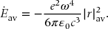
The same result is found for the analogous harmonic circular motion in the xy-plane. However, the energy of a simple harmonic oscillator is also proportional to |r|2av. Thus, the average energy loss is proportional to the negative of the energy of the oscillator. This implies that the energy decays exponentially in time,

where E0 is the energy originally available and a is the fractional decay rate. The classical weighted average loss rate over the entire duration of the radiative decay is

The corresponding decay rate is

where |r|2av is averaged over the entire duration of radiative decay.
Quantum mechanically, the weighted average value of r in the state described by the wavefunction Ψ is given by the expectation value

Here, r has been generalized to a vector. As a transition is being made, the wavefunction is a time-dependent wavefunction

Substituting into Eq. (23.50) we obtain the expectation value of r during irradiation

The analog of the classical angular frequency is

Now interpret that the value  averaged over the period of irradiation is given quantum mechanically by

from which the decay rate is

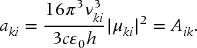
From Eq. (23.55), we see that the transition dipole moment is equal to

from which we can make the identification that the decay rate is, in fact, the Einstein A coefficient for the transition
Whereas, Eq. (23.55) was ambiguous as to whether the frequency dependence of the ratio of Aik to Bik was due to Aik, Eq. (23.57) makes it clear that it is the rate of spontaneous emission that increases with increasing transition frequency. Also from Eq. (23.55), the Einstein B coefficient is

Stay updated, free articles. Join our Telegram channel

Full access? Get Clinical Tree


