Developing quantum mechanical intuition
The world of subatomic particles simply does not behave how everyday macroscopic objects do. Because of this you will need to be introduced to numerous new phenomena and a new vocabulary. One of the best ways to be ready for the new ideas of quantum mechanics is to be comfortable with the physics of classical electromagnetic waves and classical mechanics of particles. Hence, here we first review a few items of terminology and then proceed to review wave behavior and classical mechanics.
The use of quantum mechanics is most necessary for atomic scale distances and masses. A convenient length scale is the Ångström (1 Å = 0.1 nm = 1 × 10⁻¹⁰ m), in particular because bonds are on the order of 1 Å in length. Of course, this unit is not recommended within the SI system of units; however, it is simply so convenient and widespread, it still finds use. Another non-SI unit that is extremely useful is the electron volt, eV. Covalent bond energies are on the order of several eV. The electron volt is equal to the kinetic energy of an electron (or any other particle with a charge of one elementary unit e = 1.602 × 10⁻¹⁹ C) that is accelerated through a potential difference of 1 V. Thus, the conversion factor between the clumsy (on the atomic scale) joule and the convenient electron volt is 1.602 × 10⁻¹⁹ J eV−1. The electron volt is convenient when speaking of the energy of a single subatomic particle, while kJ mol−1 is convenient when dealing with on the order of Avagadro’s number worth of particles, 1 eV = 96.485 kJ mol−1.
Spectroscopy is the primary means by which we investigate the quantum world. The interpretation of spectroscopic data is key to our understanding. Remember that spectrum is singular and its plural is spectra.
19.1 Classical electromagnetic waves
19.1.1 Characteristics of light
Light is described as an oscillation of ‘something’ at right-angles to the direction of propagation – a transverse wave. The ‘something’ that is oscillating is the amplitude of electric and magnetic fields, as shown in Fig. 19.1. They oscillate with a frequency ν and a wavelength λ. Sitting at one point in space and counting how many complete oscillations the wave makes in a given length of time is a measure of the frequency, the units of which are per unit time, s−1 or hertz (Hz). The distance between two successive maxima (or two successive minima) is equal to the wavelength, which is measured in units of distance. Maxima and minima collectively are known as extrema and also as antinodes. The sign of the oscillating field changes from (+) to (–) and passes through zero at a node. Another commonly encountered descriptor of electromagnetic waves is the wavenumber  , which is measured in inverse length, m−1 in SI. However, because it is so ingrained in the literature, the more commonly encountered unit is cm−1 and this will be used here.

Figure 19.1 (a) A classical electromagnetic wave is composed of an oscillating electric field E and a magnetic field B that oscillates perpendicular to the electric field. The z-axis is chosen to lie perpendicular to the direction of the electric field, and the electric field oscillates in the xy-plane. (b) A wave of amplitude A0 (absolute value of the maximum or minimum field strength) at the antinodes. The wavelength λ is the distance that it takes for the wave to complete a full cycle. A node is a point at which the field strength goes to zero. The sign of the electric or magnetic field changes sign on either side of a node.
The speed of light was the first physical constant to be assigned an exact value. This is because it is used as the basis for defining many other fundamental constants. The speed of light in vacuum is represented by c, and is

If we need to differentiate it from the speed of light in a medium, we will denote the speed of light in vacuum as c0 and the speed of light in a medium as c. The refractive index is the ratio between the speed of light in vacuum and the speed of light in a medium

The product of wavelength λ and frequency ν is equal to the speed of light

The wavenumber  is the inverse of the wavelength thus,

Implicit in our discussion below, and throughout this book, is that we are considering propagation of light in vacuo – that is, in a medium with refractive index n = 1. This is a simplifying approximation so that we do not have to keep track of this factor of n and label everything with a subscript 0. When light enters a dense medium, its speed decreases in proportion to the refractive index, as shown in Eq. (19.2). The electromagnetic field of light establishes a polarization in the medium that oscillates at the same frequency as the incident light. Therefore, the frequency of light in the medium remains constant at ν. However, in accord with Eq. (19.3) the wavelength of light in the medium λ must be reduced from its value in vacuo λ0 such that λ = λ0/n. The refractive index is a slowly varying function of frequency in a transparent material, but changes rapidly near absorption features. The refractive index of air is nair = 1.0003 at 589 nm (a standard wavelength associated with the familiar yellow D line emission of Na). When performing high-resolution spectroscopy it is important to correct for this factor that would change the D1 line from λ0 = 589.76 nm to λ = 589.58 nm for light propagating in air at atmospheric pressure. The refractive index is proportional to density. Therefore, it depends not only on the composition of the medium but also on temperature and pressure. For example, water at atmospheric pressure and 20 °C has n = 1.3330.
James Clerk Maxwell developed the mathematical theory of magnetic fields and showed that electricity and magnetism cannot exist in isolation. He suggested that light was composed of oscillating electric E and magnetic B fields, which are perpendicular to each other, and that these field can be represented by sine or cosine waves,


where ω = 2πν is the angular frequency (units of radians per second represented by s−1 and never Hz), and k = 2π/λ is the wavevector. The maximum values of the amplitudes of the electric and magnetic fields are E0 and B0, respectively. The argument of the cosine function is known as the phase of the wave φ0

Light propagating in a uniform medium has a constant phase. Thus, differentiating this equation with respect to time and setting it equal to zero, we obtain the phase velocity of the wave

What is commonly called the ‘speed of light’ is the speed at which a point of constant phase (an antinode, for example) propagates past a fixed observer. An electromagnetic wave is two-dimensional and c is the propagation velocity of a plane of constant phase along the x-axis.
The intensity of a classical wave is proportional to |A|2, where A is the amplitude of the wave. Thus, the intensity of an electric field (what is commonly measured in any light detector since the interaction of matter with the magnetic field is generally much weaker) is proportional to E20. φ describes the relative phase (phase difference) of the waves. The term ‘relative phase’ describes the displacement of one wave with respect to another. Waves that have constant displacement are coherent waves – that is, they are in phase with each other. Waves that are in phase add constructively, while waves that are out of phase add destructively. A shift in phase by 90° (= π/2 radians) changes a sine wave into a cosine wave

Recall that a cosine function can also be represented by a complex exponential function

and that i2 = −1. Therefore, an equivalent way to write the wave equation of the electric field is

where the relative phase φ has been included explicitly. The real part of E represents the physical wave. Using this complex notation, the intensity is proportional to the absolute square of the field, that is by the product of the complex conjugate of the field E* with the field E

Electromagnetic radiation can possess a near infinite range of wavelengths. The span of wavelengths is termed the electromagnetic spectrum; this is shown in Fig. 19.2. The electromagnetic spectrum ranges from radio waves at low energy up to cosmic rays at the high end. The length unit of choice depends on the spectral range. Different parts of the spectrum are associated not only with different names, but also with different characteristic molecular/atomic excitations as noted in Table 19.1. This means that different regions are also associated with different spectroscopic techniques, which also tend to have different preferred units. Hence, pure rotational spectroscopy often uses wavelength in μm, frequency in MHz, or wavenumber in cm−1; vibrational spectroscopy (also called infrared spectroscopy) is most commonly conducted in cm−1 but sometimes also in μm. Visible light is commonly referenced by wavelength in nm, though wavenumber in cm−1 is also used. This is true for electronic spectroscopy throughout the UV/Visible range. X-ray spectroscopy and X-ray diffraction often reference the wavelength in Å (now sometimes in pm) or photon energy in eV. Gamma spectroscopy is often performed in energy units of keV or MeV.

Figure 19.2 The electromagnetic spectrum.
Table 19.1 The electromagnetic spectrum divided into different wavelength ranges.
| Spectral range | Wavelength | Energy / eV | Excitation |
|---|---|---|---|
| Radio | 100 km–100 cm | 10−11–10−6 | nuclear spin |
| Microwave | 100 cm–1 mm | 10−6–10−3 | rotation |
| Infrared | 1 mm–700 nm | 10−3–1.8 | rotation, vibration |
| Visible | 700–400 nm | 1.8–3.1 | valence electrons |
| Ultraviolet | 400–200 nm | 3.1–6.2 | valence electrons |
| Vacuum ultraviolet | 200–100 nm | 6.2–12.4 | deep valence |
| Extreme ultraviolet | 100–10 nm | 12.4–124 | deep valence |
| X-ray | 10–0.01 nm | 125–125 k | core electrons |
| Gamma ray | <10 pm | >125 k | nuclear states |
Several other terms are commonly associated with light and electromagnetic waves. White light is comprised of waves of many frequencies. White light can be characterized by a central frequency and a broad bandwidth of frequencies of random phase on either side of this central value. This is in contrast to monochromatic light (light of a single frequency) or narrow bandwidth light (light of a small frequency range). Plane-polarized light has its E field in a well-defined plane. The plane of the E field is termed the plane of polarization. In circularly polarized light, the E field rotates in a plane orthogonal to the propagation direction.
19.1.2 Superposition of waves
In addition to oscillating with a definite frequency and wavelength, one of the essential defining characteristics of a wave is its ability to exhibit interference phenomena as a result of the relative phase behavior of combined waves. In Figs 19.3–19.5 we see the results of the superposition of two waves of equal amplitude propagating collinearly. Three different cases are shown: Fig. 19.3 shows equal frequency and in-phase; Fig. 19.4 shows equal frequency and out-of-phase; and Fig. 19.5 shows initially in-phase but unequal wavelength.

Figure 19.3 The constructive interference of in-phase waves of the same wavelength.
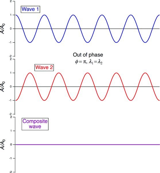
Figure 19.4 The destructive interference of out-of-phase waves of the same wavelength.

Figure 19.5 The variable interference (beat pattern) of incoherent waves – waves with different wavelengths and therefore variable phase.
All electromagnetic waves of the same wavelength travel at the same speed in the same medium. Therefore, waves of equal wavelength that are in-phase at the origin remain in phase everywhere. Note that waves with a well-defined phase relationship need to be added coherently. That is, the electric field of the combined wave is obtained by adding the electric fields of the component waves. The intensity of the combined wave is then obtained by squaring the summed wave. In a coherent sum, add waves then square to obtain the intensity.
Consider two waves that they have the same frequency and amplitude but a phase difference φ. They may be written


The electric field of the superposed wave is obtained by addition of the two waves

Factoring out a term of e− iφ/2 from the term in parenthesis and expanding the result using Eq. (19.10), we rewrite the electric field of the superposed waved as

This allows us to write E as a product of real functions and complex exponential functions only. This simplifies the result because in taking the product involving the complex conjugate,

Therefore, the intensity (irradiance) is

19.1.2.1 Directed practice
Complete the algebraic steps necessary to derive Eq. (19.18).
If the waves did not have a well-defined phase relationship, an incoherent sum would be performed. In an incoherent sum, the intensity of the each wave is first obtained by squaring the field strength, then the component intensities are added to obtain the resultant intensity of the combined wave. In a coherent sum of two waves with equal amplitude E0, the maximum intensity is 4E20. In an incoherent sum of two waves with equal amplitude E0, the maximum intensity is 2E20. The output of two conventional light bulbs adds incoherently: two 100 W bulbs have the same intensity as one 200 W bulb (avoiding for the moment any consideration of distance dependences and shadowing from the construction of the bulbs).
However, if we have coherent sources – most easily constructed from lasers but also possible with classical sources under special conditions – then we need to consider the relative phases of the constituent waves. Constructive interference is perfect for waves of the same wavelength and amplitude that are in phase φ = 0 or, more generally, differ in phase by φ = 2nπ, where n is an integer. Constructive interference becomes progressively weaker as the phase difference increases. Time invariant interference between two sources of light can only take place if they are coherent sources, that is, they must have the same frequency and have a constant phase difference.
When the phase difference increases to π radians, the interference becomes perfectly destructive for waves of the same wavelength and amplitude. This is shown in Fig. 19.4. Interference is a periodic phenomenon and destructive interference becomes increasingly less effective as the phase difference increases beyond π radians. Destructive interference is a maximum at φ = (2n + 1)π, with n again an integer.
Waves with different frequencies and a well-defined initial phase relationship display variable interference because the relative phase difference changes with time. This is shown in Fig. 19.5 and is known as a beat pattern. Note that energy is conserved. Interference leads to changes in the distribution of radiant energy. Destructive interference at the node redistributes energy into the antinodes. Interference phenomena can only occur where beams overlap and the occurrence of destructive interference at one point in space and time must be accompanied by constructive interference elsewhere to balance it. For complete destructive interference to occur at all points in time and space it would mean that the two beams would have to interfere at their sources such that no energy is radiated at all.2 We will see in Chapter 27 that fitting cycles of light inside an optical cavity such that they interfere constructively is important in the design of lasers.
If the two waves have slightly different values of wavelength described by k + Δk and ω + Δω, the total electric field that results from the two waves propagating collinearly is

This equation has the same form as Eq. (19.15) but with the relative phase difference replaced by

The superposed intensity is then described by

The cosine factor describes an envelope function that modulates the traveling waves. This traveling wave propagates with a group velocity of

This represents the velocity at which a plane of constant phase of the envelope travels. It need not be equal to the phase velocity of the individual waves.
19.1.3 Double slit interference
Pick a plane of constant phase, say a maximum, and follow it as the wave propagates. We refer to this plane as the wavefront (we could pick any plane of constant phase but the maximum is the most commonly chosen). The wavefront is normal to the direction of propagation. A plane wave is a collimated beam with plane wavefronts.
Consider the situation depicted in Fig. 19.6 in which a monochromatic plane wave is incident on two infinitesimal slits a distance d apart. Each slit acts as a point source and we observe the light transmitted from these slits on a screen at a distance L away. The electric field at point P is the sum of the fields emanating from our two sources,

where A is the amplitude and r1 and r2 are the distances of the two slits from the point P. When L is large compared to d, the paths from the two slits are effectively parallel and r1 and r2 differ by only d = sin θ, a quantity that is called the optical path difference (OPD). Therefore,

which corresponds to a phase difference between the two waves of


Figure 19.6 The geometry of the two-slit interference phenomenon. Slits that are small compared to their separation d are situated a distance L from a screen. A dark fringe is observed at the point P on a screen when the pathlength difference r2 – r1 meets the requirement for destructive interference.
The intensity is obtained from the absolute square of the electric field,

For large L, the angle θ is small and

The light incident on the screen exhibits an interference pattern that has a cos2 variation with the distance x from the origin along the screen. Maxima (instances of constructive interference) occur whenever the OPD is equal to an integral multiple of π,

and minima (instances of destructive interference) occur when

The resulting intensity pattern is shown in Fig. 19.7. The fringes do not extend to infinity in any real case because the source cannot be perfectly monochromatic and collimated (though lasers can get extremely close to this) and the slits cannot be infinitesimally narrow, lest no light pass. This second effect causes the light passing through the slits to be emitted in cones rather than hemispheres. Because of this, the intensity is damped as the distance from the origin increases.

Figure 19.7 The modulation depth of cos2 interference fringes observed in two-slit diffraction increases as d increases when the spacing is small compared to the wavelength. It reaches a limiting value at d = λ/2 at which point subsidiary maximum begin to grow in as d increases further.
19.1.4 Multiple-slit interference
If we generalize the geometry of Fig. 19.6 from one slit to N slits, we find that the OPD between rays emanating from adjacent slits is again dsin θ. The OPD between the first and the jth slit is then (j − 1)dsin θ. Summing the electric fields of the individual slits and squaring, we find the intensity of the resulting interference pattern to be given by

The large principal maximum occurs at

where m = 0, ±1, ±2, …. This is more commonly presented as the grating equation,

where m is known as the order. The grating equation predicts the angle at which different wavelengths will leave a diffraction grating. As is obvious from this derivation, a diffraction grating does not actually diffract the light. The light is subject to multiple slit interference in reflection. Interference is the result of several beams of light interacting with one another. Diffraction is more accurately defined as the interaction of light with a single aperture.
19.1.4.1 Example
Determine the angular location of the first three orders for a grating with 6000 lines cm−1 and incident yellow light with λ = 589 nm.
The first-order reflection is found at an angle given by the solution of the grating equation for m = 1, sinθ = λ /d. The distance between slits is the inverse of the ruling density, d = 1/6000 cm = 1.667 × 10⁻⁶ m. Solving for the angle, we find, sin θ = 589 × 10− 9 m/1.667 × 10− 6 m = 0.3534, which corresponds to θ = 20.7°.
Second order, m = 2, sinθ = 0.3534 × 2 = 0.7068 ⇒ θ = 45.0°
Third order, m = 3, sinθ = 0.3534 × 3 = 1.0602, an unphysical result for θ – that is, it cannot be observed with this grating.
19.1.5 ‘Diffraction’ in crystals
The lattice structure of a crystal resembles a diffraction grating where the ‘slits’ are the spaces between the ordered atoms of the crystal, as shown in Fig. 19.8. If d = 2 Å (a distance on the order of a bond length or the spacing of planes in a crystal) and sinθ = 0.3534 (which from the above example seems like a reasonable sort of angle), then the wavelength of light that would diffract into this angle is


Figure 19.8 Diffraction (actually multiple-source interference) from a series of parallel planes as in a crystal.
This is in the X-ray region.
Because of this, X-ray diffraction is used to determine the structures of crystals. Diffraction patterns are collected from crystals irradiated with X-rays of a known wavelength and spacings are found by solving the Bragg equation,

We recognize this as the grating equation, with the order now represented by n and dhkl is the spacing between planes designated by the Miller indices hkl. In Fig. 19.8, the sum of the red line segments PB and BQ represents the pathlength difference between the ray that reflects from the lattice plane at point A and the ray that reflects from the lattice plane below it at point B (similarly and successively for the planes below it). When the pathlength difference corresponds to integer values, constructive interference is observed. When it corresponds to half-integer values, the waves associated with the two rays are out-of-phase and destructively interfere with one another.
19.2 Classical mechanics to quantum mechanics
The last decade of the 19th century and first decade of the 20th century were an incredible period in science that could have benefited from a greater sense of humility. Albert Michelson, quoting Lord Kelvin, stated in 1894 that science had “… exhausted new discoveries and that advances were only to be made in more precision of measurement.” At about the same time, Ernst Mach and Wilhelm Ostwald were fighting vociferously against the idea that molecules existed. Against this backdrop one has to interpret how revolutionary Ludwig Boltzmann’s ideas of statistical mechanics and the necessity of atoms and molecules really were at the time. By 1900, Max Planck would apply statistical mechanics to demonstrate the need for the quantization of energy, specifically the quantization of oscillators to explain black-body radiation. By 1905, Albert Einstein would use Planck’s hypothesis to demonstrate that light behaves not only like a wave, but also like a particle with quantized energy. In 1907, Einstein combined statistical mechanics with quantum theory to explain the low-temperature behavior of solids. And by 1913 Niels Bohr declared his theory of quantized orbits for electrons in atoms. Our perception of the world would never be the same.
Now of course, we know that the materials around us are composed of atoms and molecules. Chemically, the world is quantized: there is a smallest unit (the atom/molecule) that is the smallest stable clump of matter with a given set of chemical properties. From Einstein, we know that energy and mass are equivalent

Therefore, since matter is ‘quantized’ in molecules why should we be surprised that energy is quantized as photons or that molecules can have quantized energy states? This is easy to say in hindsight, but it is not our experience from the classical world and macroscopic objects. We can kick a football at any speed (up to some limit fortunately for goalkeepers). We can spin in circles at any rotation rate. It is not our experience that we can only spin at angular frequencies with specified values or with our rotational axis pointed only in certain directions. Again, some perspective is in order. That is how macroscopic objects behave, and while many precepts of classical physics are still valid, subatomic and atomic particles simply behave in a manner that is different from what our senses experience.
Because we live in a world of classical physics, none of us comes to the study of quantum mechanics with quantum intuition. We possess classical intuition. In order to develop quantum intuition, we need to be ready to jettison treasured ideas from classical physics and everyday intuition. To develop quantum intuition we need to use something that looks like what we will later call the ‘variational principle.’ We need to introduce a set of terms (call them a basis set) that approximates the answers to our questions. If the approximation works well and describes our solutions to the level of accuracy that is available, then our basis set was appropriate. If the answer is not quite accurate enough, we can add a few more terms that modify our description. If the answer is way off we might try to add a few more terms. However, eventually we may need to throw out the original basis set and start with new terms and a better approximation to begin with. In other words, we will use classical analogies and push them as far as we can. But when they fail, we must be ready to accept new quantum mechanical ideas – new terms – that we add to our classical language.
With a perspective that was not available to the intrepid souls who pioneered quantum mechanics, we can aid the development of quantum intuition by stating a few principles that will remain inviolable. The laws of thermodynamics apply to quantum systems. Thus, conservation of energy still holds. Indeed, Noether’s first theorem, proven by A. Emmy Noether in 1915 but published later,3 demands that time invariance in physical laws (that is, when you perform your experiments neither changes the laws of physics nor the spectrum of hydrogen) requires the conservation of energy and linear momentum, just as rotationally symmetric physical laws require conservation of angular momentum. Causality still holds. Combined with relativity, this may lead to some very interesting paradoxes, but the application of unbalanced forces still accelerates particles. Quantum mechanics converges on classical mechanics for macroscopic objects. With this in mind, we can review a few concepts derived from classical mechanics.
Classical mechanics is based on an assumption of exact trajectories. We know where a particle is, its velocity, its mass, and therefore its momentum. The kinetic energy of a particle of mass m is

Stay updated, free articles. Join our Telegram channel

Full access? Get Clinical Tree


