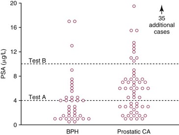
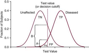
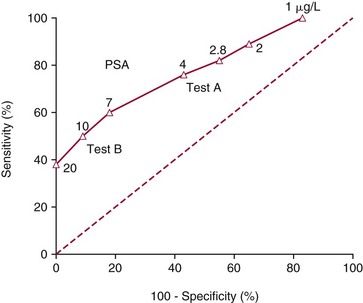
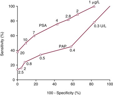
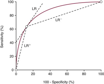
Sensitivity and Specificity

The sensitivity of a test reflects the fraction of those with a specified disease that the test correctly predicts. The specificity is the fraction of those without the disease that the test correctly predicts. Table 3-1 shows the classification of unaffected and diseased individuals by test result. True positives (TP) are those diseased individuals who are correctly classified by the test. False positives (FP) are nondiseased individuals misclassified by the test. False negatives (FN) are those diseased patients misclassified by the test. True negatives (TN) are nondiseased patients correctly classified by the test.

Both high sensitivity (few FN) and high specificity (few FP) are desirable characteristics for a test, but one is typically preferred over the other, depending on the clinical situation.

By design, some tests have only positive or negative results and provide qualitative results. These tests, which are termed dichotomous, have a single sensitivity and specificity pair for a designated assay cutoff. If a cutoff value is selected to produce high sensitivity, the specificity often will be compromised. Likewise, cutoffs that maximize specificity lower sensitivity.

An example of a dichotomous test is the human immunodeficiency virus (HIV) screening test. This test detects HIV antibodies, producing results that may be nonreactive (negative) or reactive (positive). False positives occur owing to technical errors such as mislabeling or contamination and the presence of cross-reacting antibodies found in individuals such as multiparous women and multiply transfused patients.²⁸ False negatives occur because of technical errors such as mispipetting and sampling determinants such as testing in early infection (3 to 4 weeks) prior to antibody production. Reported sensitivities and specificities for the HIV screening test vary widely,¹⁶ but reasonable estimates are 96% and 99.8%, respectively. Thus, 4 of 100 HIV-infected subjects will test negative. Only 2 of 1000 noninfected subjects will test positive. The clinical usefulness of an HIV test result from an unknown subject will be explained later in the “Probabilistic Reasoning” section.

As opposed to dichotomous tests, continuous tests are those that produce quantitative results. Continuous tests have an infinite number of sensitivity and specificity pairs, as the cutoff varies from lowest to highest decision value.

Figure 3-1 is a dot plot of the performance of a continuous assay for prostatic-specific antigen (PSA) in patients with benign prostatic hyperplasia (BPH) and in those with established carcinoma of the prostate (stages A through D).⁸ Often continuous tests are used in a dichotomous fashion by choosing one or more decision cutoffs. Note the two dashed lines crossing the graphs that represent two diagnostic cutoffs. Both tests A and B are PSA tests, but they have different decision cutoffs, namely, 4 µg/L and 10 µg/L. When test A is compared with test B, the decision cutoff of 4 µg/L for test A produces increased sensitivity but at the cost of a decrease in specificity. Thus increased true-positive detection has been traded for an increase in the number of false-positive results. This tradeoff occurs in every test performed in medicine. Not only does it affect the interpretation of quantitative laboratory results, it also affects the opinions of surgical pathologists and radiologists and of the care provider who performs a physical examination.

Figure 3-2 illustrates a hypothetical test that shows higher results in patients who have a disease compared with those who are unaffected. As the decision cutoff is increased, FP decrease and FN increase. At extremely low and extremely high cutoffs, sensitivity and specificity are 100%.

Receiver Operating Characteristic Curves⁴⁸

The dot plot (see Figure 3-1) displays quantitative performance in a limited fashion. For example, one cannot easily estimate sensitivity and specificity for various decision cutoffs using the dot plot. A graphical technique for displaying the same information, called a receiver operating characteristic (ROC) curve, began to be used during World War II to examine the sensitivity and specificity associated with radar detection of enemy aircraft. An ROC curve is generated by plotting sensitivity (y-axis) versus 1 − specificity (x-axis).^10a

Figure 3-3 shows the ROC curve for the data in Figure 3-1. The x-axis plots the fraction of nondiseased patients who were erroneously categorized as positive for a specific decision threshold. This “false-positive rate” is mathematically the same as 1 − specificity. The y-axis plots the “true-positive rate” (the sensitivity). A “hidden” third axis is contained within the curve itself: the curve is drawn through points that represent different decision cutoff values. Those decision cutoffs are listed as labels on the curve.¹⁸ The entire curve is a graphical display of the performance of the test.

Tests A and B from Figure 3-3 are displayed as two decision points on the ROC curve. The dotted line extending from the lower left to the upper right represents a test with no discrimination and is designated the random guess line. A curve that is “above” the diagonal line describes performance that is better than random guessing. A curve that extends from the lower left to the upper left and then to the upper right is a perfect test. The area under the curve describes the test’s overall performance, although usually one is interested only in its performance in a specific region of the curve.¹ One strength of the ROC graph lies in its provision of a meaningful comparison of the diagnostic performance of different tests. In the medical literature, the use of 2 × 2 tables to present the sensitivity and specificity of a test has led to the common logical misconception that a quantitative test has a single sensitivity and specificity. When the initial publication of an assay recommends a cutoff for analysis purposes, the assay is often categorized as sensitive or specific based on this cutoff. Yet, as seen in the ROC curve, every assay can be as sensitive as desired at some cutoff, and as specific as desired at another.

When two procedures are compared, confusion is avoided by using ROC curves instead of accepting statements such as, “Test A is more sensitive, but test B is more specific.” For example, the usefulness of the prostatic acid phosphatase assay had been compared for years with that of the PSA assay for diagnostic and follow-up purposes. Various claims were made regarding the relative sensitivity and specificity of the two assays.12,35

Figure 3-4 compares the performance of an acid phosphatase assay with that of the PSA assay for discrimination between BPH and prostatic carcinoma in the same cohort of patients. Although each test has been claimed to be “more sensitive but less specific” than the other by various authors, it is clear from the ROC curves that the authors were choosing different points on the two curves. No matter what level of sensitivity is chosen, the PSA assay offers greater specificity than the acid phosphatase assay at the same level of sensitivity. This does not mean that one should conclude that the PSA assay is always superior. It does indicate that for the cohort of patients used to compare the assays, the PSA assay offers superior performance compared with the prostatic acid phosphatase assay. However, the acid phosphatase assay may provide superior diagnostic information to that provided by the PSA assay in subpopulations of the cohort.

The area under the ROC curve is a relative measure of a test’s performance. A Wilcoxon statistic (or equivalently, the Mann-Whitney U-test) statistically determines which ROC curve has more area under it. These methods are particularly helpful when the curves do not intersect. When the ROC curves of two laboratory tests assessing for the same disease intersect, the tests may exhibit different diagnostic performances, even though the areas under the curve are identical. Test performance depends on the region of the curve (i.e., high sensitivity vs. high specificity) chosen. Details on how individual points on two curves can be compared statistically have been provided elsewhere.¹

Prevalence

Prevalence is defined as the frequency of disease in the population examined.⁴⁴ For example, with step sectioning of prostate tissue from a random sample of men older than 50 years of age, at least a 25% probability of histologic carcinoma is expected (most of the carcinomas identified will never become clinically important, but they are carcinomas nevertheless).^17,34 Several useful techniques have been applied to combine the prevalence with information previously obtained in the results of testing.

Predictive Values

The results of dichotomous tests (and continuous tests used in a dichotomous manner) can be interpreted using predictive values. The predictive value of a positive test (PV⁺) is the fraction of subjects with a positive test who have the disease. The predictive value of a negative test (PV⁻) is the fraction of subjects with a negative test who do not have the disease. The predictive value equations are as follows:

Predictive values are a function of sensitivity, specificity, and prevalence. It is regrettable that clinicians often confuse sensitivity with PV⁺. For example, suppose that 1,000,000 U.S. residents were randomly chosen and tested for HIV infection using the HIV screening test. The Centers for Disease Control and Prevention estimates that the prevalence of HIV infection in the United States is 330.4 per 100,000 population.⁷ On the basis of this prevalence, about 3304 infected individuals would be expected in a population of 1 million. Because the sensitivity of the HIV test is 96%, about 3172 infected individuals would have a positive test result (i.e., TP = 3172). Similarly, because the specificity of the HIV test is 99.8%, about 2 false positives per 1000 subjects would be expected. Thus about 1993 individuals would have false-positive results (i.e., FP = 1993). Therefore, the PV⁺ is 3172/(3172 + 1993), or 61%. Thus an individual with a positive test result has a moderate chance of having a false-positive result. Additional testing is necessary to separate TP individuals from FP individuals. Most laboratories automatically test all specimens having a positive HIV screening result with a confirmatory test such as the HIV Western blot (see Chapter 12).

In this example, the PV⁻ is much higher than the PV⁺. Calculations reveal 132 false-negative results (3304 − 3172) and about 994,703 true negatives [99.8% × (1,000,000 − 3304)]. Thus, the PV⁻ is 99.987%. Note that many of the false negatives could reflect these infected individuals with early HIV infection prior to antibody development. The limitation of false negatives can be overcome by frequent testing of high-risk individuals.

Odds Ratio

The odds ratio (OR) is defined as the probability of the presence of a specific disease divided by the probability of its absence. The odds ratio reflects the prevalence of the disease in a population. For example, the probability of occurrence of a 1.3-cm³ carcinoma in a 75-year-old man is about 8%. The odds ratio of finding histologic carcinoma measuring greater than 1.3 cm³ after the prostate is sectioned from the autopsy specimen of a man older than 70 years is thus 0.08/(1 − 0.08), or 1 to 11.5. Findings from a digital rectal examination, from transrectal ultrasonography, or from both consist of other data that affect the previous probability of the presence of prostatic disease.

Likelihood Ratio

The likelihood ratio (LR) is the probability of occurrence of a specific test value given that the disease is present divided by the probability of the same test value if the disease was absent. Many sources (e.g., Henry²⁰) indicate that the slope of the ROC curve is equal to the LR for a given test value. Assertions such as these oversimplify the concept of LR. Choi¹⁰ describes three different slopes of the ROC curve, which represent LR in different settings (as illustrated in Figure 3-5):

For qualitative tests, the positive likelihood ratio (LR⁺) is equal to the sensitivity/(1 − specificity). Conversely, the negative likelihood ratio (LR⁻) is the probability of occurrence of a specific test value given that the disease is absent divided by the probability of the same test value if the disease were present. Thus for qualitative tests, the LR⁻ is specificity/(1 − sensitivity).

For quantitative tests, the LR is the tangent slope of the ROC curve, which equals the ratio of the heights A and B of the two curves at the test value in Figure 3-2. Note that the areas under each curve in Figure 3-2 are the same. The likelihood ratio does not take disease prevalence or any other prior information into account. To arrive at a final probability, one must adjust for the best estimate of the probability of disease before obtaining the test result.