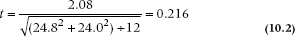
. So the test, called a paired t-test, is equal to:

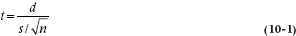
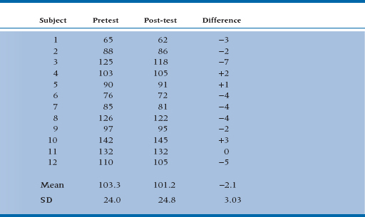
TABLE 10–1 Pretest and post-test weights of 12 Casimir subjects

In this case, it equals .

Now, the critical value of a one-tailed t-test with 11 df (12 data − 1 mean) at the .05 level is equal to 1.80. Casimir will undoubtedly proclaim to the world that the C¹¹ diet is “scientifically proven” and cite papers to back up his claim. Of course, you recall Chapter 6 and are a little more suspicious of one-tailed tests.

For illustration, if we were intent on randomizing to two groups at all costs, we could have gone ahead with an independent sample t-test. For the sake of argument, assume that the pretest values were instead derived from a control group of 12 who were destined to pass up the benefits of the curry plan. If they must maintain their wicked ways, it is likely that they would be the same as the treatment group before the treatment began. We could then compare the treatment group after treatment to the control group with an independent sample test as we did in Chapter 8:

Given all the previous discussion, you should not be surprised to see that this t-test is minuscule and doesn’t warrant a peek at Table C in the Appendix.

Therein lies the power of repeated observations. In the situation where small differences resulting from treatments are superimposed on large, stable differences between individuals, it can’t be beat.

So why do all these randomized trials, where folks are assigned to one group or another and measured at the end of the study? There are three reasons, all of which go against the simple paired observation design: one a design issue, one a logistic issue, and one a statistical issue. We’ll take them in that order.

The design problem is that a simple pretest–post-test design does not control for a zillion other variables that might explain the observed differences. Maybe the local union went on strike and the study subjects had to cut back on the food bill. Maybe “20/20” came out with a new Baba Wawa piece on the beneficial effect of kiwi fruit for dieters.⁴ All of these are alternative “treatments” that might have contributed to the observed weight loss. For these reasons, most textbooks on experimental design mention this design only to dismiss it out of hand.

The logistic problem is more complicated. In many situations a pretest is not possible or desirable. If the outcome is mortality rates, it makes little sense to measure alive/dead at the beginning of the study. If it is an educational intervention, it is often dangerous to measure achievement at the beginning because the pretest measurement may be very much a part of the intervention, telling students what you want them to learn as well as anything you teach to them. Or it may be far too costly to measure things at the beginning.

Finally, there is a statistical issue. If no large, stable between-individual differences exist, not only will you not gain ground with a paired comparison, but you could possibly lose statistical power. The reason is that the difference score involves two measurements, each with associated error or variability. Comparing groups on the basis of only post-treatment scores introduces error from (1) within-subject variation and (2) between-subject variation. Taking differences introduces within-subject variation twice. If within-subject variation exceeds between-subject variation, the latter test will have less power than has the former.

To illustrate this point a bit more, and also to confront the design issue, let’s consider a slightly more elaborate design. As we indicated, the difficulty with the pre-post design is that any number of agents might have come into play between the first and second measurement, and we have no justification for taking all the credit. One obvious way around the issue is to go back to the classical randomized experiment: randomizing folks to get and not get our ministrations, and then measuring both groups before and after the treatment. Now the data might look like that in Table 10–2.

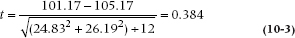
First of all, this is not exactly a classic randomized controlled trial; that would only measure weights after treatment and then compare treatment and control groups with an unpaired t-test. The calibrated eyeball indicates that such a test is not worth the trouble; the mean in the treatment group is 101.17 kg and in the control group is 105.16 kg. The difference amounts to 4 kg, but the SDs are about 25 kg in each group. Nonetheless, for completeness, we’ll go ahead and do it.

However, an alternative approach that takes advantage of the difference measure is to simply ask whether the average weight loss in the treatment group is different from the average weight loss in the control group.⁵ If we call the weight loss Δ, the null hypothesis comparing treatment (T) and control (C) groups is:

Having framed the question this way, the obvious test is an unpaired t-test on the difference scores:

TABLE 10–2 Pretest and post-test weights of 12 Casimir subjects and 12 controls

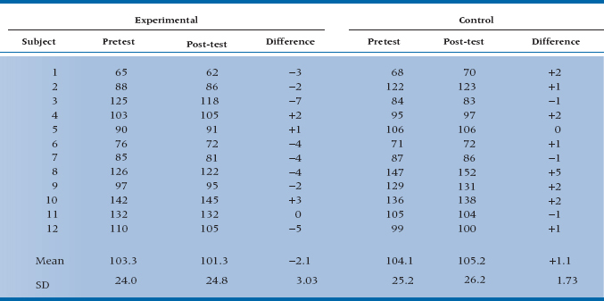
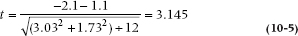
This is significant at the .05 level (t[22] = 2.07). The test of significance for the difference score is considerably higher than is the t-test for the post-test scores, even though the absolute difference was smaller (3.2 instead of 4.0), because the between-subject SD (about 24 to 26) is much larger than the within-subject SD (1.7 to 3.5).

OTHER USES OF THE PAIRED T-TEST

The example that we just used, of testing the effect of the C¹¹ diet by measuring people before and after an intervention, is probably the most common way that the paired t-test is used. But, there are other situations where the paired t-test is not only handy, but mandatory. One problem with the study of teaching Academish 1A7 we described in Chapter 7 is that we’re trusting randomization to result in both groups being similar at baseline in their ability to say “hegemonic phallocentric discourse” and other such phrases without breaking into uncontrollable peals of laughter. Randomization works in the long run (say, an infinite number of people per group, which would make the lecture hall quite crowded), but is no guarantee of group similarity for smaller studies. We also know that gender has an effect on language,⁶ as does area of specialization⁷ and perhaps a couple of other factors, such as age. We could improve the design by selecting people from the pool of controls by matching each person to someone in the experimental group of the same age, gender, and from the same academic department, thus insuring that the groups are relatively similar at the beginning.

Why can’t we just charge ahead and use a Student’s t-test? The reason is the same as the rationale for using the paired t-test in the C¹¹ example; subject 1 in the experimental group is, because of the matching, much more similar to subject 1 in the control group than to any other, randomly selected person. So, the situation is closer to that of one person being tested under two different conditions than of two unrelated people in different groups. We lose power if we ignore the similarity, in much the same way that we lose power if we treat a repeated measures design as if it consisted of two different groups.

But, there’s a caveat. We also lose degrees of freedom, as we just discussed in the C¹¹ example. We hope that this is more than compensated for by the reduction in between-subject variance, but this means we have to select our matching variables carefully. If subjects are matched on variables that are unrelated to the outcome, such as eye color or height, then the df is reduced with no gain in variance reduction.

EFFECT SIZE

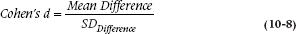
When we discussed the ES for the independent t-test in Chapter 7, we mentioned that there are a few choices, which vary in terms of which estimate of the SD is used in the denominator. Similarly, there are four ways to calculate a d-type effect size for a paired t-test, and which one you use depends on what assumptions you’re willing (or are forced) to make (Kline, 2004). Although some of these have their roots in the standard statistical literature, others have been reincarnated in a slightly different guise in clinical research (often with the authors being unaware of the index’s previous life), primarily in the form of responsiveness to change, which has been suggested in the quality-of-life literature as an important measurement characteristic, right up there with reliability and validity (e.g., Kirshner and Guyatt, 1985; but see Streiner and Norman, 2014, for the truth of the matter). Since it’s in the latter domain where you’re most likely to encounter these things, we’ll show you the parallels.

The reason there’s more than one coefficient relates directly back to the previous section, where we discussed the difference between the paired and unpaired t-tests. When you calculate an ES with paired (usually pre-post) data, you can use either the SD between people measured either before or after the intervention, or the SD within people (i.e., the SD of the differences, SD_Difference). While it usually makes little sense in a statistical test to use the SD between people in the measurement of an ES,⁸ both are defensible; they’re just different. If you use SD_Between in the denominator, you’re comparing average change with the variability among people (i.e., the treatment effect is large enough to move a patient up 1 SD). If you use SD_Difference, you’re looking at average change compared with the variability of possible changes (Norman et al., 2006).

As we’ll see, even that doesn’t exhaust the possible permutations. Using the comparison with SD_Between, the first we’ll look at is called Hedges’s g and is simply:

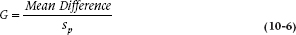
where s_p is the pooled SD from the two conditions (pre and post) or the two matched groups. The problem is that this formula assumes homogeneity of variance, and this may not be the case if the intervention changes the variance,⁹ or the two matched groups have different variances.

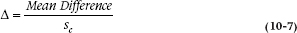
The second approach, called Glass’s Δ, gets around this by using only the preintervention or the comparison group’s SD (s_c).¹⁰ This avoids one problem, but the penalty is that the estimate of the SD is based on only half the number of observations, so it may be less accurate.

A third possibility, recommended by Cohen (1988) for pre-post designs, is to use the SD of the difference score. This has been reincarnated in the quality-of-life literature by Liang (2000) and McHorney and Tarlov (1995) and is often called the Standardized Response Mean.

If you’re comparing the change in the treatment group with the change in the control group, as in the example shown in Table 10–2, then things get more complicated. You can use (a) the pooled SD_Difference of both groups (which uses all the data but doesn’t recognize the confounding with treatment mentioned in rubric 9); (b) the SD_Difference of just the control group (Guyatt’s responsiveness) which ignores the interaction with treatment; or (c) the SD_Difference of the treatment group, which is likely the least biased measure, but uses only half the data.

What’s the relation between the two families of coefficients? Well, if there were no correlation between the pretreatment and post-treatment scores, the SD_Difference would just be s_p. In fact, though, there often is a substantial correlation, which has the effect of reducing the SD_Difference relative to s_p. (If the correlation were 1, then everyone’s postintervention score would be just the baseline score plus a constant, and the SD_Difference would be 0.) The relationship between the two SDs is:

A long stare at this equation yields an important insight that goes beyond just how to compute an ES. As we’ve already indicated, if the correlation is 1, then SD_Difference is 0, and you’re way further ahead to use difference scores in the design, since the paired t-test is infinite. If the correlation is 0, then the SD_Difference is larger than s_p, and you actually lose ground by using change scores. In fact, the equation shows that the break-even point is a correlation of 0.5; above that you’d do better to use change scores, below and you’re actually further ahead to just look at post-treatment scores.

Just remember when you use Equation 10–8 that the ES is given in units of the SD of the difference score, not in the SD of the original scale. To avoid confusion, it’s probably best to report both. In all cases, we still use the same criteria: an ES of 0.2 is small; 0.5 is moderate; and 0.8 is large.

THE CALIBRATED EYEBALL

In Chapter 7, we presented three rules for an eyeball test of significance for two independent groups, simply by plotting the means and 95% CIs. Here’s the fourth rule, applicable to the paired t-test:

(4) DON’T DO IT!

The reason is that we’re not interested in the CIs around the individual means, but rather the single CI around the difference score. The problem is that the width of this difference CI (wd) depends on the correlation¹¹ (r) between the pretest and post-test scores:

the higher the correlation, the smaller w_d. Because we can’t see that correlation by just eyeballing the data, comparing the CIs of the two means is meaningless (Cumming and Finch, 2005).

SAMPLE SIZE CALCULATION

Sample size calculations for paired t-tests are the essence of simplicity. We use the original sample size calculation introduced in Chapter 6:

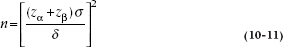
where δ is the hypothesized difference, σ is the SD of the difference, and z_α and z_β correspond to the chosen α and β levels. The only small fly in the ointment is that we must now estimate not only the treatment difference, but also the SD of the difference within subjects—which is almost never known in advance. But look on the bright side—more room for optimistic forecasts.

REPORTING GUIDELINES

Would you be surprised if we said they’re exactly the same as for the unpaired t-test that we told you about in Chapter 7? If you are surprised, go back and reread both chapters.

SUMMARY

The comparison of differences between treatment and control groups using an unpaired t-test on the difference scores (between initial and final observations, or between matched subjects) is the best of both worlds—almost. The basic strategy is to use pairs of observations to eliminate between-subject variance from the denominator of the test. The test is used in pre-post designs, and a variant of the strategy is useful in the more powerful pre-post, control group designs.

The advantage of the test exists as long as the subjects or pairs have systematic differences between them. If this is not the case, then the test can result in a loss, rather than a gain, in statistical power.

EXERCISES

1. As we discussed, at least three kinds of t-tests can be applied to data sets—unpaired t-tests, paired t-tests, and unpaired t-tests on difference scores. For the following designs, select the most appropriate.

a. Scores on this exercise before and after reading Chapter 10.

b. Crossover trial, with joint count of patients with rheumatoid arthritis, each of whom undergoes (1) 6 weeks of treatment with gold, and (2) 6 more weeks with fool’s gold (iron pyrites). Order is randomized.

c. School performance of only children versus children with one brother or sister.

d. School performance of younger versus older brother/sister in two-child families.

e. School performance of older brother/ sister in one-parent versus two-parent families.

f. Average intelligence of older and younger siblings, reared apart and reared together.

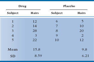
2. You may recall that we did a t-test on hair restorers in Chapter 7. Let’s return to the data, but add a piece of information: subjects were related. Subjects 1 and 6, 2 and 7, and so on are brothers. How does this change the analysis?

How to Get the Computer to Do the Work for You

• From Analyze, choose Compare Means → Paired-Samples T Test
  
• Click on the two variables to be analyzed from the list on the left [e.g., the before and after scores], and click the arrow to move them into the box marked Paired Variables
  
• Click

¹ It’s not really that simple. You know you have become obsessed with the problem when you spend a few minutes each day exploring different positions of feet, arms, and so on to see what results in minimum weight. Actually, we have found that leaving one foot off the scale works better; leaving both feet off works best of all.

² Showing off our Canadian bilingualism, this bizarre word is printed on many scales, but means, literally, “have some weight.” We sure do.

³ It’s the same reason that mad dogs and Englishmen go out in the noonday sun and is also the origin of that classic ex-pat line “There’s nothing like a nice cuppa tea (pronounced TAY) on a hot summer day.”

⁴ Who can forget the great grapefruit diet? Seduce the population, make zillions of dollars off the suckers, take a mistress who then shoots you full of holes, and lose about 5 pounds instantly as the blood drains away. And you never gain the weight back!

⁵ Of such things, Nobel prizes are not made. Nor are we implying that this is something you might not have thought of yourself.

⁶ So does sex, but we’re not allowed to discuss that in a book of this nature.

⁷ Have you ever tried to have a conversation with a business major?

⁸ Actually, as we’ll see at the end of this chapter, sometimes it makes a great deal of sense.

⁹ Which is highly likely. Different people respond differently to treatment, so the SD of the post-test is usually larger than the SD of the pretest (assuming treatment increases a person’s score).

¹⁰ Note that here, Δ is the name of a test, whereas in other circumstances it is used to represent the difference between groups. Similarly, d can either be another symbol for the difference between groups, or it can refer to a class of ES estimates. For that reason, we’re using “mean difference” rather than d in the formulae. As you can see, statistics is a rigorous way of eliminating confusion and ambiguity.

¹¹ We’ll define correlation formally in Chapter 13. Suffice it to say for now that it’s a measure of relationship; are high pretest scores associated with high post-test scores?

Stay updated, free articles. Join our Telegram channel

Join