Tests of Significance for Ranked Data
Data that can be ranked (ordinal data) should be treated differently from categorical data. This chapter reviews several ranking tests—the Mann-Whitney test (or Wilcoxon Rank Sum test) for two independent groups, the Kruskal-Wallis One-Way Analysis of Variance (ANOVA) for more than two groups, and the Wilcoxon Signed Rank test and Friedman Two-Way ANOVA for paired data.
SETTING THE SCENE
You heard that clam juice works wonders for psoriasis. Going one better, you arrange a randomized trial of Bloody Caesars (reasoning that the booze will ease the physical and psychic pain while the clam juice works its miracles). At the end, a bunch of dermatologists examine photographs of the patients and put them in rank order from best to worst. How, Dr. Skinflint, will you analyze this lot?
All academics are slaves of the publish or perish syndrome,1 and in some the illness is more acute than in others. One easy way to get big grant money (thereby ingratiating yourself to the administration) as well as publication, is to do trials of look-alike drugs or combination drugs for companies. In the present chapter, we discuss one such trial.
Dr. Skinflint, a locally renowned dermatologist, recalls reading somewhere that clam juice works wonders for the misery of psoriasis.2 He speculates that a combination of clam juice and ethyl alcohol might ease the symptoms while reducing the lesions. So he arranges a randomized trial of Bloody Caesars (BC) against Virgin Marys (VM).3 At the conclusion of the trial, he photographs all the patients and places the pictures together in random order, then he distributes the set of photos to a group of dermatologists, who are asked to simply rank the pictures from best to worst. The idea then is to examine the ranks of the patients in the BC group against the patients in the VM group.
A comment on the rank ordering. We know a couple of possible alternative approaches to measurement. The photographs could be placed on an interval scale by, for example, measuring the extent of body surface involvement. However, this might not adequately capture other aspects, such as the severity of involvement. Moreover, this could lead to a badly skewed distribution: many patients with only a small percentage of body surface area involved, and a few patients in which nearly all the skin is involved can bias parametric tests. Alternatively, some objective staging criteria, such as is used for cancer, might be devised, but this would simply lead to another ordinal scale, which must be analyzed by ranking individual subjects. Similarly, rating individuals on 7-point scales would be regarded by some (but not us) as ordinal level measurement, thus requiring non-parametric statistics. For all these reasons, proceeding directly to a subjective ranking may well represent a viable approach to measurement.
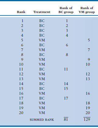
The question is now how to analyze the ranks, which are clearly ordinal level measurement. We cannot use statistics that employ means, SD, and the like. To clarify the situation, if 20 patients were in the trial, the ranks would extend from 1 (the best outcome) to 20 (the worst). If the treatment were successful, we would expect that, on the average, patients in the BC group would have higher ranks (lower numbers) than those in the VM group. Suppose Table 23–1 shows the data. It is evident that treatment has some effect. If no effect occurred, the BCs and the VMs would be interspersed, and the average rank of the BCs and the VMs would be the same. This does not seem to be happening; the BCs appear to be systematically higher in the table than do the VMs. The question is how one puts a p value on all this.
TABLE 23–1 Ranks of 20 psoriasis patients treated with BC and VM
| Rank | Treatment |
| 1 | BC |
| 2 | BC |
| 3 | BC |
| 4 | BC |
| 5 | VM |
| 6 | BC |
| 7 | VM |
| 8 | BC |
| 9 | VM |
| 10 | VM |
| 11 | BC |
| 12 | VM |
| 13 | VM |
| 14 | BC |
| 15 | BC |
| 16 | VM |
| 17 | BC |
| 18 | VM |
| 19 | VM |
| 20 | VM |
BC = Bloody Caesars; VM = Virgin Marys.
TWO INDEPENDENT GROUPS
For this simple case with two groups, several approaches are possible. Characteristically, as with many tests based on ranks, they are “cookbook-ish,” and it is nearly impossible to synthesize individual tests into a coherent conceptual whole, as we did (or think we did) with parametric tests. Fortunately, many, such as the Median test and the Kolmogorov-Smirnov test, have now faded into well-deserved obscurity. We will examine only one test, the Mann-Whitney U test. However, to make things more confusing in this particular situation, the Mann-Whitney test is also called the Wilcoxon Rank Sum test.
The test focuses on the sum of the ranks for the two groups separately, which explains Rank Sum, but not U. Anyway, as you see in Table 23–2, the calculation is the essence of simplicity. The summed rank for the BC group is 81 and for the VM group, 129. (Actually we didn’t have to calculate the second one for two reasons: (1) the sum of all ranks is N(N + 1) ÷ 2 = 210, so we can get it by subtraction, and (2) we don’t need it anyway.) The larger the difference between the two sums, the more likely the difference is real. The next step is easier still—you turn to the back of the book4 (as long as the sample size per group is less than 10) and look up 81. You find that the probability of a rank sum (W or U, depending on where your allegiance lies) as low as 81 is .0376 (using a one-tailed test), so Dr. Skinflint can get his publication after all.
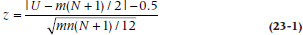
What do you do if there are more than 10 per group? Believe it or not, parametric statistics rear their heads yet again. It turns out that the normal distribution and z-test can be used as an approximation. If the total sample size is N and m are in the higher ranked group, then the expected value of the rank sum is m(N + 1) ÷ 2, or 105. So we can construct a z-test with a numerator of the observed rank sum minus the expected rank sum. The question is the form of the denominator, the SE of the difference. This turns out, after much boring algebra, to equal 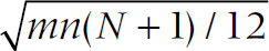 , where m and n are the two group sizes, with m + n = N. The z-test (with a continuity correction) then equals:
TABLE 23–2 Ranks of 20 psoriasis patients treated with BC and VM
BC = Bloody Caesars; VM = Virgin Marys.
which is this case is:
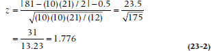
Looking this value up in Table A (in the Appendix) of the normal distribution, we find that a z of 1.776 results in a one-tail probability of .0379, very close to the tabulated value up above. As is frequently the case, nonparametric tests are devised because of a concern for bias in the parametric tests. However, except for some limiting cases, the parametric test turns out to be quite a precise approximation.
Needless to say, Dr. Skinflint (and we) are delirious that the test was significant, but is the difference between the groups large or small? What we need is an index of effect size (ES), and one exists, called the probability of superiority or, more pedantically, the measure of stochastic superiority (Vargha and Delaney, 2000). It’s abbreviated as A and is defined as:
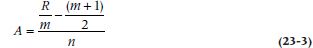
where R is the sum of the ranks for one of the groups; it doesn’t matter which one. In this example, focusing on the VM group, we have:
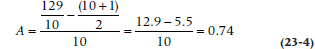
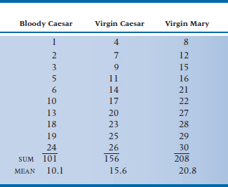
TABLE 23–3 Ranks of patients in the BC, VC, and VM trial
We can interpret that to mean that the probability of a randomly selected person in the VM group having a higher rank than one in the BM group (plus half the chance that the ranks will be equal) is 74%. If the two treatments gave identical results—equally good or equally bad—A would be 0.50, which is equivalent to Cohen’s d (the measure of ES for continuous variables) of 0.0. A d = 0.20 (a small ES) is equivalent to an A of 0.56; d = 0.50 (a moderate ES) is the same as A = 0.64; and d = 0.80 (a large ES) equals an A of 0.71 (Grissom, 1994).
MORE THAN TWO GROUPS
Following our usual progression, we can next consider the extension to three groups—the equivalent of one-way ANOVA. The strategy is a lot like the Wilcoxon (Mann-Whitney) test. However, instead of examining the total rank in each group, we calculate the average rank. And instead of doing a t-test on the ranks, we do a one-way ANOVA on the ranks. Once again, terms such as N (N + 1) and factors of 12 start kicking around, simply because of the use of ranks.
The test is another two-man team like Mann and Whitney, Kolmogorov and Smirnov, or Rimsky and Korsakoff.5 This time it’s the Kruskal-Wallis One-Way ANOVA. To illustrate, suppose we throw an intermediate group into our original design. They are fed just clamato juice, what might be called a Virgin Caesar (VC), to see whether the vodka is having any real beneficial effect on the skin of the BC group as opposed to that group’s souls. We now have 30 patients, and in Table 23–3 we have shown the ranks of the patients in each group. It is clear that these contrived data are working according to plan: the BC group has a mean rank of 10.1; the VC group, a mean rank of 15.6; and the VM group a rank of 20.8. If no difference existed, we would have expected that the average rank of each group would be about halfway, or 15. (Actually, it’s (N + 1) ÷ 2 = 15.5, because the ranks start counting at 1.) But is it significant?
To address the question (cued by the title of the test), obviously, the first thing to do is to calculate a mean square (between groups), exactly as we have been doing since Chapter 8. This looks like:
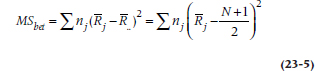
where nj is the sample size in each group; ![]() the group mean; and
the group mean; and ![]() the overall mean. So in this case it equals:
the overall mean. So in this case it equals:
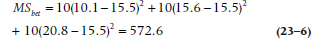
In the normal course of events, we would now have to work out a mean square (within), but because of the use of ranks again, this takes a particularly simple form: N(N + 1)/12. Writing the equation slightly differently to show what it looks like using the sums rather than the means of the ranks for each group, the final ratio (the Kruskal-Wallis, or K-W,6 test) looks like:
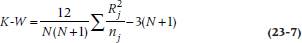
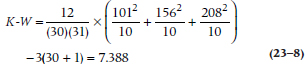
So what we end up with is:
Strictly speaking, this value should be divided by yet another equation that corrects for the effects of ties; in essence, making K-W a bit larger and hence more significant. But we’re not going to show it to you for two reasons: first, because the computer does it quite well, thank you; and second, unless there are more than about 25% of the numbers that are tied, the effect of the corrections is negligible.
For small samples, the K-W test statistic has to be retrieved from the back of someone else’s book. However, if more than five subjects are in each group, then it looks like a chi-squared distribution with (k − 1) df, where k is the number of groups. Because you shouldn’t have fewer than five subjects per group anyway, you don’t need the special table.
Multiple Comparisons
When we discussed the one-way ANOVA, we listed a large number of post-hoc analyses that are used when we find a significant F-ratio. Fortunately, or not, there’s only one such test for the Kruskal-Wallis. Any difference between mean ranks is significant if it’s larger than:
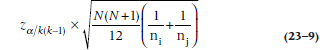
where k is the number of groups.
For the data in Table 23–3, since k(k − 1) = 6 and we’re using the traditional α of 0.05, we look up a z value of (0.05 ∴ 6) = 0.0083 in the table of the normal distribution and find it’s about 2.39. So, we’re looking at a critical value of:
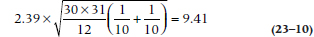
The only difference that’s larger than this is between Bloody Caesar and Virgin Mary (20.8 − 10.1), so only it is statistically significant.
Effect Size
OK, a significant difference, but how big is it? We use a variant of the A statistic from Equation 23–3 (Vargha and Delaney, 2000):
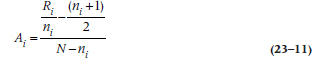
where Ri and ni are the sum of the ranks and the sample size for one of the groups. We won’t bother to go through a calculation, because it’s just the same as for the Mann-Whitney. The interpretation is similar, too, but it’s now the probability that a person randomly selected from group i has a rank larger than people from the other two groups pooled.
ORDERED MEDIANS: THE JONCKHEERE TEST
The K-W test is similar to the one-way ANOVA in that we just toss the data into the computer, press the right button, and wait to see what differences emerge. For our purposes, and for the tests to be significant, it doesn’t matter if the ordering of the groups is A > B > C, or B > A = C, or any of the other possible combinations; as long as at least two groups differ significantly, we declare victory, shut the lab down for the rest of the day, and go to the local watering hole to celebrate. But there are times when our theory lets us make more precise predictions, and we can use more powerful tests. If we believe that both clam juice and vodka have healing properties, then we’d predict that clam juice + vodka (BC) would be better than clam juice alone (VC), and that clam juice would be superior to a drink that has neither ingredient (VM). As long as our data are at least ordinal, we can use the Jonckheere Test for Ordered Alternatives (abbreviated as J) to test for this.7
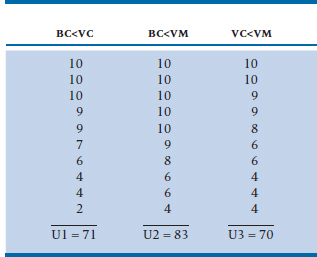
We begin by arranging the groups in the hypothesized order of their medians or mean ranks, from lowest to highest. It’s important to keep in mind that the ordering must be based on our a priori hypothesis; it’s intellectually dishonest to first look at the results, and then arrange the groups in order of their observed medians or mean ranks. Fortunately for the publisher, Table 23–3 is already in the predicted order, so he doesn’t have to spend any more (of our) money printing the table again. The next step is simple, but tedious. For each entry, we count how many values in the succeeding groups are higher. So, for subject 1 in the BC group (Rank = 1), there are 10 higher values in the VC group and 10 in the VM group. For the last subject in that group (Rank = 24), there are 2 higher values in VC and 4 in VM. We do this for all people, and the results are presented in Table 23–4. There are three things to notice about the table. First, if we have k groups, then there will be k × (k − 1) ∴ 2 columns. Second, it’s a lot easier to do this if the numbers in each column are in rank order; and finally, the bottom row is the sum of the values.
To compensate us for all the counting we had to do, the J test itself is the essence of simplicity; we just add up all the values of U:

which in this case is 224. But our luck doesn’t last too long. To test the significance of J, we use a z-like test, so we have to figure out the mean and variance of J. The mean is:
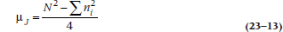
TABLE 23–4 The number of times a score from Table 23–3 is smaller than scores from succeeding groups
the variance is:
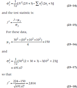
which we look up in a table of the distribution of the normal curve. Because the hypothesis is an ordered one, we use a one-tailed test, so that the critical value for α = .05 is 1.645, rather than the more usual 1.960. Since J* is larger than this (it actually corresponds to a p level of .0025), the test is significant.
TWO GROUPING FACTORS
We’re getting there. Not only have we extended the rank sum tests to include multiple groups, we have also proven, more or less, that booze is good for psoriasis (that’s the beauty of fictitious data!). However, we are still limited to one factor only. In any case, if we were setting out to examine the independent and possible interactive effects of vodka and clam juice, a much better design from the outset would be a two-factor one. To be precise, we would have four groups—clam juice and vodka (Bloody Caesar), clam juice only (Virgin Caesar), vodka only (Bloody Mary), and neither (Virgin Mary).8 We lay on the pepper and tabasco so no one can tell which is which anyway, and we again have dermatologists rank the outcomes, this time for 40 patients.
Unfortunately, it is at this point that tests on ordinal data grind to a screeching halt. Given the simple strategy used by all in this chapter, it would seem such a simple trick to take the equations of Chapter 8 and diddle them a bit for rankings. We can see it all now … “The Streiner-Norman Two-Way ANOVA for Independent Samples.” Better still, why don’t you do it, and we’ll get back to writing books?
REPEATED MEASURES: WILCOXON SIGNED RANK TEST AND FRIEDMAN TWO-WAY ANOVA
The final step in this walk through the ranked clones of the parametric tests is to consider the issue of matched or paired data—the equivalent of the paired t-test and repeated-measures ANOVA. For this excursion, let’s take the issue of clones to heart.
Suppose some cowboy scientist, Gene Auful, was let loose in the university molecular biology lab and managed to create some clones of graduate students from samples of blood they unwittingly donated to the Red Cross. The little darlings were raised by foster parents, and in due course, 20 years later, the clones end up as graduate students in the same labs (the experiment is working!). Recognizing that here are the makings of the ultimate nature-nurture experiment, one of the measures we put in place is a measure of achievement and likelihood of success, arrived at by getting the graduate faculty to sit around a table with all the files of both original and clone students and ranking them.9 One measure of successful clones would be that they, on the average, are ranked just as highly on ability to succeed. The data are in Table 23–5.
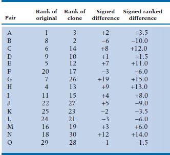
There are 15 pairs, and we have listed the rank order of the original and the clone, ranging from 1 to 30, where (this time) 1 is best and 30 is worst. It seems that the clones are actually a bit inferior because their average rank appears higher than that of the originals. This is confirmed in the fourth column, which is the first step to the Wilcoxon Signed Ranks test (wasn’t he a busy little lad!), where we have calculated the difference of ranks for each pair. Next, we rank the differences in column five, so that the smallest differences have the first rank (ignoring the sign, but carrying it through). You will notice some funny-looking numbers in the right column. We have three 6s, two 2.5s, and two 1.5s, but no 5s, 7s, or 1s. The problem is caused by having three differences of 3, which should take up the ranks of fifth, sixth, and seventh; two differences of 2, which should be third and fourth; and two differences of 1, which should be first and second. Because we don’t know which is which, to avoid any infighting, we give them all (or both) the average rank: 6, 3.5, or 1.5.
Finally we sum the ranks of the positive and negative differences. The positive sum is (3.5 + 12 + 1.5 + 11 + 15 + … + 14) = 84, and the negative sum turns out to be 36; as before, they sum to N (N + 1) ÷ 2 = 120.
Now, under the null hypothesis that no difference exists between original and clone, we would anticipate that the average rank of the originals and the clones would be about the same. If so, then the differences between rankings would all be small, and the sum of the rankings for both the positive and the negative differences would be small. If either of the summed differences is large, this indicates a substantial difference between the average original rank of the individuals in the matched pairs and so would lead to rejection of the null hypothesis.
Once again, we rush expectantly to the back of the book, only to be disappointed. However, in Siegel and Castellan (1988), a T of 84 (that’s what the sum refers to) is not quite significant (p = .094). And once again, the table stops at a sample size of 15 matched pairs. For larger samples there is (you guessed it) an approximate z-test, based on the fact that, once again, this statistic is approximately normally distributed, with a mean and SD based on the number of pairs, N. The formula is:
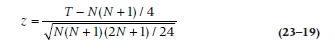
In the present case, z equals 1.842, and the associated p-value is .066, not quite the same as the exact value calculated from the table, but close enough.
The A-type measure of effect size for a repeated measures or matched-pairs design is so simple we’re not even going to give you a formula. It’s merely the proportion of difference scores that are positive. In Table 23–5, 10 of the 15 scores are positive, so the probability is 0.67 that a person drawn at random will have a higher score on the second occasion. We told you it would be simple.
The extension of this test to three or more groups, the equivalent of repeated-measures ANOVA, is the Friedman test. We won’t spell it out in detail because (1) it follows along a familiar path of summed ranks, and (2) the applications are rare. Briefly, it considers matched groups of three, four, or however many, each of which is assigned to a different treatment. It calculates the rank of each member of the trio or quartet. If one treatment is clearly superior, then that member of the group would be ranked first every time. If another treatment is awful, the member receiving that treatment would always come in last. And if the null hypothesis were true, all the ranks would be scrambled up. You then calculate the total of the ranks under each condition and plug the average ranks into a formula, again involving sum of squares and Ns. For a small sample, you look it up in a table; for a large sample, you approximate it with an F distribution. For more information, see Siegel and Castellan, yet again.
SAMPLE SIZE AND POWER
We did Medline, Statline, PsychInfo, and Edline searches, and we even called a few 1–900 numbers, but we were unable to come up with any formulas for sample size calculations on rank tests.10 What should we do if the granting agency demands them? Determine the sample size from the equivalent parametric test (e.g., t-test, one-way ANOVA, paired t-test), and leave it at that. For a long time, it was assumed that nonparametric tests were less powerful than parametric ones, so some people (us, for example, in the first edition) suggested adding a “fudge factor.” More recent work, however, has shown that you don’t lose any power with these tests and, when the data aren’t normal, they may even be more powerful than their parametric equivalents.11
TABLE 23–5 Ranking of graduate students and their clones on success
SUMMARY
In this chapter, we dealt with several ways to do statistical inference on ranks. We should remind you that, although the examples used rankings as a primary variable, in circumstances where the distributions are very skewed or the data are suspiciously noninterval, such as staging in cancer, the data can often be converted to ranks and analyzed with one of these nonparametric tests.
Why not use ranking tests all the time and avoid all the assumptions of parametric statistics? The main reason is simply that the technology of rank tests is not as advanced (there really is no Streiner-Norman two-way ANOVA by ranks), so the rank tests are more limited in potential application. A second reason is that they tend to be a little bit conservative (i.e., when the equivalent parametric test says p = .05, the rank test says p = .08); however, they are not nearly as conservative as are tests for categories such as chi-squared when applied to interval-level data.
For two groups, we used the Wilcoxon rank sum test, also called the Mann-Whitney U test. For more than two groups, we used the Kruskal-Wallis one-way ANOVA by ranks. For matched or paired data, Wilcoxon arrived on the scene once more, with the Wilcoxon matched pair signed rank test,12 and the Friedman test was briefly described as an extension to more than two groups.
EXERCISES
1. Is it really true that “Gentlemen Prefer Blondes?” To test this hypothesis, we assemble 24 Playboy playmate centerfolds from back issues—8 blondes, 8 brunettes, and 8 redheads. To avoid bias from extraneous variables, we use only the top third of each picture. We locate some gentlemen (with great difficulty) and get them to rank order the ladies from highest to lowest preference.
The data look like this:
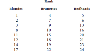
Proceed to analyze it with the appropriate test.
2. In retaliation, the ladies decide to do their own pin-up analysis to address another age-old question related to the encounters between the sexes (oops—genders). Is it true that bald men are more sexy? To improve experimental control over the sloppy study done by the gents, they work out a way to control for all extraneous variables. They go to one of those clinics that claim to make chromedomes into full heads of hair and get a bunch of before-after pictures. They get some ladies to rank the snapshots from most to least sexy and then analyze the ranks of the boys with and without rugs. It looks like this:
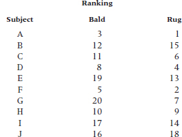
Go ahead and analyze this one too.
3.One last kick at the cat. The gentlemen, most of whom are predictably thinning, express displeasure at the results of the ladies’ study, and assault it on methodological grounds (naturally). They claim that men who would go and buy rugs are not representative of all bald men. So the ladies proceed to repeat the study, only this time ripping out Playgirl centerfolds (top third again), and getting ranks. Now the data look like:
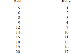
Analyze appropriately.
How to Get the Computer to Do the Work for You
All of the procedures follow the same format, so we won’t bother to go into detail for each of them. The statistic you want, in every case, is the default option. They all start off the same way:
From Analyze, choose Nonparametric Tests
Then select the appropriate option for the desired test
Mann-Whitney U (Wilcoxon Rank Sum Test)
2 Independent Samples
Kruskal-Wallis one-way ANOVA
K Independent Samples
Wilcoxon Signed Rank Test
2 Related Samples
Friedman Two-Way ANOVA
K Related Samples
Jonkheere’s Test
Forget it; you’ll have to do it by hand.
1 One disciple to another while taking Christ from the cross: “He was a great teacher, but he didn’t publish.”
2 “Somewhere” was in the preeminent international oeuvre, PDQ Statistics.
3 For the teetotalers in our midst (both of them!), a Bloody Caesar contains tomato juice, Tabasco, clam juice, and vodka. A Virgin Mary is missing the clam juice and alcohol.
4 Some books, not this one. We recommend Siegel and Castellan (1988) for all nonparametric tests. As we’ll see in a minute, though, we really don’t need the tables.
5 Of course, these days a hyphenated name stands for one married woman, not two men. Probably reflects the observation that one woman can do about as much as two men anyway. Certainly, because most of these seem to be a simple adaptation of a parametric test developed by one man, one wonders why it took two to do it.
6 Unlike most other statistical tests, which have widely accepted letters that label them (e.g., F, t, or r), K-W is left out in the cold. Siegel and Castellan (1988) use KW; Bewick and colleagues (2004) use T; and we’re using K-W in order to assert our individuality.
7 Perhaps the most difficult aspect of this test is how to pronounce it. It’s “Young Care.”
8 Lest you are offended by the labels, these are all legitimate drinks, and can be purchased in any reputable bar (and many disreputable ones).
9 You know now this is a fictitious example. Professors never agree on anything. Clark Kerr (UCSF) once said that, “A university is a collection of scholars joined by a common heating system.”
10 However, a few of the 1–900 numbers gave us suggestions for other things, which can’t be mentioned in this family-oriented book.
11 If you need some references for the grant and are loath to cite us, use Blair and Higgins, 1985, or Hunter and May, 1993; or, if you want to appear more up-to-date, Zimmerman, 2011.
12 By the time you finish the title, you know what the test does.
Stay updated, free articles. Join our Telegram channel

Full access? Get Clinical Tree


