This distribution provides probability rule for the realisation of r heads out of n tosses. The constant p is the parameter of this distribution, which is the actual probability of one success. A second example is a normal distribution

This distribution provides probability rule for the realization of values of y when the distribution of y has a bell shape. The constants µ and σ² are the parameters of this distribution. Parameter µ is the real mean value of y and σ² is the real variance of y. The symbol ‘~’ is used to denote a distribution. For example, X~N(µ, σ²) indicates, X has a normal distribution with mean µ and variance σ². As mentioned above, in general, the values of parameters are unknown. However, since a sample is assumed to imitate the population, some estimations of these parameters are possible using the observed sample values. These estimates of parameters are known as statistics. An estimate may be only a single number describing a possible value of the associated parameter (point estimate), or an interval describing a probability that the parameter will be in that interval (interval estimation). In the following section, we will discuss estimation procedure of some common parameters.

Descriptive Statistics

Descriptive statistics are summary values of the observed sample. These summary values attempt to describe the characteristics of the associated population parameters. Some common descriptive statistics are mean, median, mode, moment (or more specifically p^th moment about A, defined below), variance, standard deviation, standard error, mean deviation, etc. In this discussion, the symbol will represent sum of n observed x values. For example, if x has 5 values as x₁ = 1, x₂ = 4, x₃ = 4, x₄ = 6, and x₅ = 7, then = 1 + 4 + 4 + 6 + 7 = 22. Using this notation we define, sample mean . Mean is generally denoted by µ for population and for sample. Population mean of a variable X is also known as the expected value of X and is denoted as E(X). Median is the middle value of the observed sample values in magnitude. For its calculation, we first arrange the observed sample values in ascending order and pick the middle value in case of odd number of observations, and mean of middle two observations in case of even number of observations. Median is generally denoted by M for population and m for sample. Mode is the observation that is repeated most number of times. For its calculation, find how many times each observation is repeated. Pick the one that has highest repetition. An observed sample may have no mode or more than one modes. The p^th sample moment about A is defined as .

Moment is generally denoted by µ_p for population and by m_p for sample.

Sample variance =

where is the mean of observed x values.

Note that variance is the 2^nd moment about mean. Variance is generally denoted by V or σ² for population and by v or s² for sample. Standard deviation = . Standard deviation is generally denoted by SD or σ for population and by sd or s for sample. Coefficient of variation CV = and the corresponding estimate is cv = Note that CV is a unit free value of standard deviation relative to the mean. Since CV is unit free, it is convenient to compare the variation of different variables in terms of CV.

Sample mean deviation =

generally denoted by MD for population and md for sample. The m^th percentile denoted by p^m is defined as a value of the observed sample so that m% of the observations is less than this value and (100–m)% observations are greater than this value. The value p²⁵ is known as the first quartile (Q₁) and the value p⁷⁵ is known as the third quartile (Q₃). Therefore, there are 25% observations smaller than Q₁ and 75% of observations are greater than Q₁. Similarly, there are 75% observations smaller than Q₃ and 25% of observations are greater than Q₃. The second quartile Q₂ = p⁵⁰ is the same as the median. The difference IQR = Q₃ – Q₁ is known as the interquartile range. The SAS Proc univariate and Proc means provide some of these summary statistics.

Since a statistic is a function of the observed sample values, it is a random variable, that is, it varies from sample to sample. Therefore, it also has a distribution with some parameters. The distribution of a statistic is known as sampling distribution. For example if X ~ N(µ, σ²) then the sample mean ~ N(µ, σ²/n), that is, has a normal distribution with mean = µ and variance = σ²/n. The square root of this variance is the standard deviation of . In the statistical literature the standard deviation of a statistic is known as standard error (S.E.) of the statistics. Therefore, correctly has a distribution with mean = µ and S.E() = An estimate of this S.E. is

Example 1: Suppose plasma concentrations of a test substance in 10 animals have the following values, x = 4, 2, 1, 3, 5, 6, 5, 3, 6, 3. The calculated summary statistics (using SAS Proc univariate) are as follows: = 3.8, sd = 1.69, Median = 3.5, Mode = 3.0, CV = 44.38, Mean deviation = 1.40 and p⁷⁵ = 5.

Sometimes more than one variable is measured from the same experimental unit. For example, the height, weight and blood pressure may be measured for each subject in the experiment. For such data, two important summary statistics are covariance and correlation coefficient. Both of these statistics measure the pairwise dependency of one variable on another. The correlation coefficient is the standardised value of covariance and is unit free. Therefore, the correlation coefficient is easy to interpret compared to covariance. The population correlation is generally denoted by ρ(x, y) or simply by ρ, while this for sample is denoted by r(x,y) or simply by r. These two summary statistics are calculated as follows.

Suppose x and y are two variables measured from same experimental unit, then the sample covariance

and the correlation coefficient

where n is the number of observations. It can be shown that the value of r is in (–1 to 1). A positive value of r implies a direct relation between x and y, that is, as x increases y also increases and vice versa. A negative value of r implies a reverse relation between x and y, that is, as x increases y decreases and vice versa. A value of r = 1 implies a perfect correlation between x and y with direct relation between x and y. In this case a graph between x and y falls on a straight line with positive slope. Whereas a value of r = –1 implies a perfect correlation between x and y with reverse relation between x and y. In this case a graph between x and y falls on a straight line with negative slope.

Example 2: Consider the following dataset obtained for age-related changes in plasma immunoglobulin M (IgM) level after immunisation determined in Wistar rats. The observed values are shown in Table 17.1. The details of the calculations of covariance and correlation coefficient are given in Table 17.2.

Number of observation, n = 11.

Table 17.2. Calculation of covariance and correlation coefficient

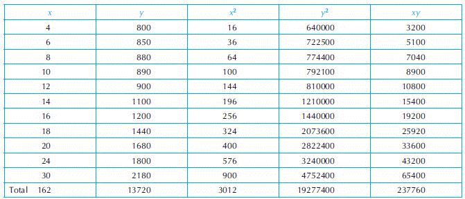
Results show that age and immunoglobulin have almost a perfect correlation. The SAS Proc corr can provide these estimates of covariance and correlation.

Estimations and Confidence Intervals

As mentioned before, the values of parameters are generally unknown. Some estimations of these parameters are possible using the observed sample values. In general, a sample proportion is the estimate of population proportion, sample mean is the estimate of population mean, sample variance is the estimate of the population variance, etc. For example, if we assume that the 10 observations in Example 1 are from a normal distribution N(µ,σ²), then the estimate of µ is calculated from the 10 observations, and estimate of variance σ² is s² calculated from the 10 observations. Sample estimates should have some desired properties, for example, unbiasedness, consistency, efficiency, sufficiency. Due to limitation of space, these properties will not be discussed here. Statistically, an estimate with more of these properties is assumed to be better.

Since a statistics is a function of the observed sample values, it is a random variable, that is, it varies from sample to sample. Therefore, a point estimate may be very close or far from the real value of the associated parameter. This difference cannot be enumerated by such a single value. An alternative to this point estimate is an interval estimate. This estimate calculates two values known as lower (l) and the upper (u) limits in such a way that the actual value of the parameter will be within these limits with a high probability. The interval defined by these two limits is known as the confidence interval, C.I.= (u,l). For example, if X is distributed as N(µ, σ²) then l = and u = are the lower and the upper limits for the (1 – α)% confidence interval for µ. In a different notation, the (1 – α)% C.I. for µ is . However, to be more accurate from t-distribution with n – 1 degree of freedom (d.f.) should be used instead of that is, . The (1 – α)% C.I. for σ² is l = and u = , where is the χ² value with n – 1 d.f. with α/2% tail to the left, and is the χ² value with n – 1 d.f. and (1 – α/2)% tail to the left.

The interpretation of this confidence interval is that if the calculation of confidence interval is repeated 100 times by taking sets of 100 independent samples using the above formula, then (1 – α)% times the actual value of µ is expected to be captured by the calculated intervals. If α = 0.05 then z_1–α/2 = 1.96 is the 97.5% tail probability of standard normal distribution z~N(0.1). In this case the calculated confidence interval is known as the 95% confidence interval. Theoretically, confidence intervals can be calculated for any parameter. However, for some parameters the process may be quite complicated.

Example 3: Consider observations 3.9, 4.2, 4.2, 3.8, 3.6, 4.4, 4.1, 3.4, 4.0, 3.5, 3.7 and 4.2 came from N(µ, σ²). Suppose that both population mean µ and variance σ² are unknown and we would like to calculate an 80% confidence interval for the mean µ.

We have

Thus,

From t-table t_0.9,11 = 1.363 and the 80% confidence interval on µ is

Suppose µ₁ and µ₂ are population means from two populations. Also let x₁, …, x_m, and y₁, …, y_n be two samples for these two populations. The (1 – α)% confidence interval on the difference of these means µ₁ – µ₂ can be found as

Where s_p =

Central Limit Theorem

If x₁, x₂, …, x_n is a sample of size n from a population not necessarily normal with mean µ and variance σ², Then for large n, the sample mean has approximately a normal distribution with mean µ and variance σ²/n. In notations we say, as . This property of large sample is known as the central limit theorem. As a consequence of this theorem, statistical tests (discussed in a later section) originally meant for normal population are also applicable to non-normal populations for large sample.

Statistical Hypothesis Testing and Sample Size Calculation

Statistical Hypothesis Testing

As pointed out earlier, population parameters are generally unknown. However, sometimes they may have hypothetical values. It is sometimes possible to test if such hypothetical values of parameters are true using a representative sample observation from this population. This statistical procedure of verification is known as the test of hypothesis. Since we deal with the parameters of a population, the procedure is known as parametric method. In later part of this section we will discuss test of hypothesis not regarding parameters of any population. The procedure then will be called non-parametric method.

Formally, we first express a hypothetical true value of the parameter in the form of a hypothesis, known as the null hypothesis (H₀), and possible other values of the parameter in the form of an alternative hypothesis (H₁). In notations, H₀: θ = θ₀ and H₁: θ > θ₀ or H₁: θ < θ₀ (both of these are known as one-sided alternative) or H₁: θ ≠ θ₀ (known as two-sided alternative) where θ denotes a parameter. The general idea is to calculate the difference or ratio r = between the estimate of the parameter and the corresponding hypothetical value and make a determination on the validity of the hypothetical value of the parameter based on the magnitude of this difference or ratio. A big absolute value of d indicates the falsehood of the null hypothesis and a small value of d indicates truthfulness of the null hypothesis. Similarly, a small or large value of r indicates the falsehood of the null hypothesis and a value of r very close to 1 indicates truthfulness of the null hypothesis. An important component of this process is the selection of a cut-off point on d (or r) to decide on the truthfulness or falsehood of the null hypothesis. For this purpose the difference (or the ratio) is standardised. This standardised value is known as test statistic (Z). A cut-off point is then determined based on the distribution of this statistics. There are two types of errors associated with this process, known as the Type 1 and Type 2 errors. They are defined in Table 17.3.

Table 17.3. Type 1 and type 2 errors

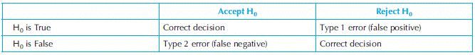
These two error types are enumerated by percent of times they happen.

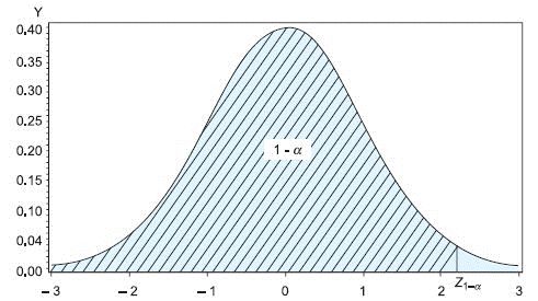
The Type 1 error is generally denoted by α and the Type 2 error is generally denoted by β. We want these errors to be as small as possible. The cut-off point for the test is generally fixed such that the Type 1 error is less than a pre-specified value. This cut-off point is known as the critical value and the corresponding Type 1 error (α) is known as the test level. Generally α is set to 5% or 1%. The value (1 – β) × 100 is known as the power of the test. There are two operational criteria to draw conclusion in a hypothesis testing known as (i) critical value criteria and (ii) p-value criteria. In the first criteria, for one-sided alternative with H₁: θ > θ₀, compare z with the critical value z_1–α. If the calculated statistic z is greater than the critical value z_1–α, reject the null hypothesis, accept otherwise. For one-sided alternative with H₁: θ < θ₀, compare z with the critical value z_α. If the calculated statistic z is less than the critical value z_α, reject the null hypothesis, accept otherwise. The critical values z_1–α and z_α are taken from standard tables. For two-sided alternative, compare |z| with the critical value z_1–α/2. In the second criteria, for one-sided alternative H₁: θ > θ₀, calculate the p-value defined as p = P(Z > Z_1-α). If this calculated p-value is smaller than the test level α reject the null hypothesis, accept otherwise. For one-sided alternative H₁: θ < θ₀, calculate the p-value defined as p = P(Z < z_α). If this calculated p-value is smaller than the test level α reject the null hypothesis, accept otherwise. For two-sided alternative, calculate the p-value defined as p = P(|Z| > Z_1–α/2). If this calculated p-value is smaller than α/2 reject the null hypothesis, accept otherwise. Clearly the two criteria are equivalent (Figure 17.1).

Figure 17.1. Normal density curve.

Sample Size Calculation

For any statistical hypothesis both Type 1 and Type 2 errors are sensitive to the sample size. In general, as the sample size becomes large both Type 1 and Type 2 errors become small. However, as the sample size becomes large, the cost, time and complexity of conducting the experiment grow. Therefore, for any experiment, a reasonable sample size is desirable. In practice, an acceptable Type 1 error and an acceptable Type 2 error are first determined and then the sample size is calculated to satisfy these two requirements. There are mathematical formulas that can calculate a sample size satisfying the required Type 1 and Type 2 errors. Because of the limitation of space, the derivation procedure of these mathematical formulas has not been discussed.

An example of these mathematical formulae for testing a single mean is as follows. Consider testing the hypothesis H₀: µ = µ₀ against the alternative H₁: µ = µ₁. Suppose that the intended Type 1 error = α and Type 2 error = β, then the sample size n that satisfies these requirements is calculated using the formula

where z_(1-α) and z_(1-β) are the (1 – α)% and (1 – β)% tail values of z, respectively. For example, consider a test with, H₀: µ = 370 against H₁: µ = 365. Assume σ = 20, α = 0.025, and β = 0.05 or power = 95%. We have z_{(1 – α)} = 1.96 and z_{(1 – β)} = 1.64. Therefore,

Thus, to perform a 0.05 level test for null hypothesis, H₀: µ = 370 against H₁: µ = 365 with a power of 95% we need a sample of about 208 subjects.

Also, for test for equality of two population means, with equal sample size from each population, we have the following formula. The null hypothesis H₀: µ₁ = µ₂ and the alternative hypothesis . Suppose that the intended Type 1 error = α and Type 2 error = β, then the sample size n (from each population) that satisfies these requirements is

Presently, many statistical software packages are available to calculate the sample size under different conditions and requirements. Some of these softwares are nQuary, Power analysis, Sample size calculator, PASS, EAST, SAS, etc. These softwares are generally simple to use and highly accurate.

In the following sections we will discuss the test procedure for some common parametric and non-parametric methods for test of hypothesis.

Parametric Method

Test for Single Proportion

Assumptions: The inherent population is binomial with parameter p. The test level = α.

Observation: Sample x₁, x₂, …, x_n of size n, where each x_i is either 0 or 1.

Null hypothesis: H₀: p = p₀.

Alternative hypothesis: H₁: p > p₀ (one-sided alternative).

Test statistic

Conclusion: Reject H₀ if where is the percentile of standard normal distribution (Z). If the alternative is H₁: p < p₀ then reject . If the alternative is two-sided, that is, H₁:p ≠ p₀. Reject H₀ if (two tail test), where is the percentile of z.

Example 4: In an experiment 5 female mice were given a special diet to study its effect on the gender of their pups. During the study period there were 5 litters with a total of 32 pups (12 males and 20 females). The null hypothesis is that the diet did not affect the gender of the pups. Let p represent the proportion of males. If diet does not have any effect on gender, then p should be 0.5. Therefore, we have H₀: p = 0.5 and H₁: p < 0.5, n = 30, = –1.0954. From normal table, we have z_0.05 = –1.64. Since –1.0954 > z_0.05 we accept the null hypothesis, that is, the treatment did not have any effect on the gender of the pups.

Test for Two Proportions

Assumptions: The inherent populations are binomial. The test level = α.

Observation: Sample 1, x₁, x₂, …, x_m of size m, and Sample 2, y₁, y₂, …, y_n of size n where each x_i and y_j are either 0 or 1.

Null hypothesis: H₀: p₁ = p₂.

Alternative hypothesis: .

Test statistic:

where is the pooled estimate of variance of p. The is calculated as

Conclusion: Reject H₀ if where is the 1-α/2 percentile of t distribution with m + n – 2 degrees of freedom. If sample sizes are large alternatively reject H₀ if where z_1-α/2 is the 1-α/2 percentile of z.

Example 5: Consider an example in which two treatments were applied on two groups of animals to evaluate the effect of treatment on survival. At the end of the experiment there were 425 deaths out of 500 animals in Group 1, and 459 deaths out of 500 animals in Group 2. We would like to test the equality of the proportions of deaths in the two treatment groups at test level 0.05. The null hypothesis is, H₀: there is no difference between two treatments with regard to survival of animals.

Since sample size is very large we can use z test. From normal table z_0.975 = 1.96. Since 3.35 > z_0.975 we reject the null hypothesis and conclude that there is a statistically significant difference in survival of animals in the two treatment groups.

Test for Dose–Response Relationship (Trend) of m Incidence Rates (m Proportions)

Cochran-Armitage Test: Consider an experiment in which 40 animals were randomly but equally divided into four groups. Group 1 was control. Groups 2, 3 and 4 received, respectively, low, mid and high doses of an experimental drug. At the end of the treatment the presence and absence of a certain disease was observed. Table 17.4 shows the data.

Table 17.4. Number of animals with disease

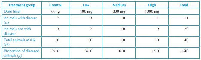
Our interest is to test the dose–response relationship (trend) of incidence rates of the diseased animals. The null hypothesis is, H₀: there is no dose–response relationship on the proportions of diseased animals. The Cochran–Armitage test statistic is defined as the following:

where x_i is the i^th dose, n_i is the number of animals with disease in the i^th dose group, N_i is the number of animals at risk in the i^th dose group, The statistic χ² has a χ² distribution with 1 degree of freedom. The critical value χ_α,(1)² can be obtained from the χ² table.

Example 6: For the data in the above table χ² = 11.06, with α = 0.05 the critical χ²_0.95,(1) value is 3.84. Since 11.06 > χ²_0.95,(1), we reject the null hypothesis (that there is no dose–response relationship) and conclude that there exists a statistically significant dose–response relationship in the proportions of diseased animals.

Test for Single Mean

Assumptions: The inherent population is normal. The test level = α.

Observation: Sample x₁, x₂, …, x_n of size n.

Null hypothesis: H₀: µ = µ₀.

Alternative hypothesis: H₁: µ > µ₀.

Test statistic: if σ² is known and is unknown

where s =

Conclusion: Reject H₀ if is known, and is unknown, where z_1-α is the 1–α^th percentile of z distribution, is the 1–α percentile of t distribution with n – 1 d.f., which can be obtained from a t-table. If the alternative is two-sided, for example , reject H₀ if is known, and if σ² is unknown.

Example 7: Suppose we have the following 10 observations from an experiment: 10.2, 11.0, 12.8, 10.8, 11.1, 9.9, 12.1, 10.2, 11.6 and 11.4. We would like to test the hypothesis H₀: µ = 11 against the alternative H₁: µ > 11 with lest level α = 0.05. The population variance σ² is assumed to be unknown. We have n = 10,

From the table 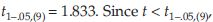we accept the null hypothesis and conclude that the population mean, from which the sample came, is 11.

In the above discussion the population was assumed to be normal. Therefore, before applying this test it is necessary to test the normality assumption of the population. Several descriptive methods can be used to check for normality. A brief description of some of these methods is as follows:

1. Construct a histogram of the data and check the shape of the graph. If the data came from a normal distribution, the histogram will be bell shaped.

2. Compute intervals and determine the percentage of observations falling in each. If the data are approximately normal, the percentages will be approximately equal to 68%, 95% and 99%, respectively.

3. Find the interquartile range IQR = Q2 – Q1, and standard deviation s, from the sample. Calculate the ratio IQR/s. This ratio should be close to 1.3 for approximately normal population.

4. Construct a normal probability plot (or a normal plot) for the data. If the data are approximately normal, this plot will be approximately a straight line. To construct a normal plot, order the observations from the smallest to the largest, calculate the corresponding expected z-score. Plot the ordered observations against the expected z-scores. To calculate the expected z-score for the m^th ordered observation x_(m), calculate the percentage p_m of observations bigger than x_(m). Find the value z_(m) of z (from standard normal table or some software) such that P(z > z_(m)) = p_m. This z_(m) is the z–score for x_(m).

Example 8: An example of drawing a normal plot is as follows. Suppose we have 11 observations 36.3, 32.7, 40.5, 36.2, 38.5, 36.3, 41.0, 37.0, 37.1, 39.9 and 41.0. We want to plot a normal probability plot (Figure 17.2). Calculations are shown in Table 17.5.

Table 17.5. Observed values and expected normal variates

Figure 17.2. Plot of EZ against Y.

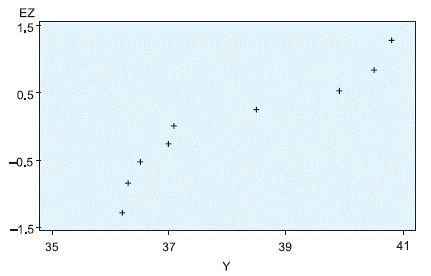
The plot does not look like a straight line. Therefore, the observations do not appear to be coming from a normal population. However, in this example the sample size is too small. For an accurate conclusion the sample size needs to be reasonably large.

Test for Equality of Two Means from Two Populations

Assumptions: The two inherent populations are normal with equal variances. The test level = α.

Observation: Sample x₁₁, x₁₂,… of size n₁ from Population 1 and x₂₁, x₂₂,… of size n₂ from Population 2.

Null hypothesis: H₀: µ₁ = µ₂.

Alternative hypothesis: H₁: µ₁ > µ₂.

Test statistic: z = if the common variance σ² is known, and

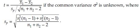
Conclusion: Reject H₀ if z ≥ z_1-α if the common variance σ² is known, and if the common variance σ² is unknown, where z_1-α is the 1-α percentile of z distribution and is the 1-α percentile of t distribution with n₁ + n₂ – 2 d.f. If the alternative is two-sided, for example reject 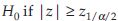if the common variance σ² is known, and 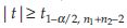if the common variance σ² is unknown.

Example 9: Suppose we have 60 observations from each of the two populations with mean vales of µ₁ and µ₂, respectively. Suppose the common population variance σ² is unknown. Let following be the summary statistics from the samples: The null hypothesis H₀: µ₁ = µ₂, and alternate hypothesis , also let α = 0.05. We have,

From table t_0.975,(158) = 1.96. Since t > t_0.975,(158) = we reject H₀, that is, we reject µ₁ = µ₂.

In the above discussion, the variances of the two populations were assumed to be equal. Therefore, before applying this test it is necessary to test the equality of the population variances. A test for the equality of variances is given in a later section. If the test reveals that the population variances are not equal, the problem is popularly known as the Behrens-Fisher problem. In this case the test statistic is defined as

and the degrees of freedom is estimated as

Test for Equality of Several Means

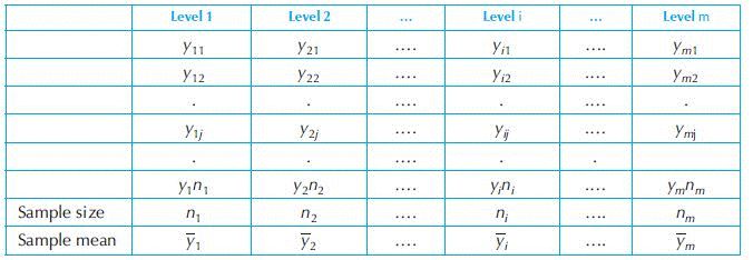
Before describing the test procedure for several means, we need to discuss a statistical technique known as analysis of variance. The discussion will be very brief. A complete description of this topic needs much deeper statistical discussion which is outside the scope of this chapter. The interested readers are referred to the book by Hogg and Tanis.¹ Suppose m different doses of a drug are tested on m groups of similar patients. The drug is expected to be effective and change the disease level. The data may be written as shown in Table 17.6.

Table 17.6. Data layout for several dose levels experiment

Stay updated, free articles. Join our Telegram channel

Join