(20.1)
i.e. the sum of the values of the variable (xi) considered, divided by the number (n) of elements in the population. If the population is very large or infinite, its mean can only either be estimated from a random sample taken from the population, or its value can be derived from probability theory e.g. the mean of the standard normal distribution is by definition zero. The calculated sample mean (m),

(20.1a)
Observed values of a population or sample show as a rule a certain degree of variation around the mean. There are a number of options to quantify this variation.
Observations or measurements are said to be accurate if they are unbiased estimates (Sect. 20.2.1) of the corresponding true value, and are said to be precise (or reproducible) if their replicated measurements have low variation. See Fig. 29.1 in chapter Basic Operations for a schematic representation of accuracy and precision.
The term accuracy often is incorrectly used as precision is meant and sometimes accuracy means accuracy and precision together. To avoid misunderstandings, it is recommended to use the terms accuracy and precision in their proper meaning (see Sect. 32.16.6).
One option to quantify variability is to draw a graphical representation of the frequency of certain values of the property concerned, called a histogram. The values are divided into classes.
Figure 20.1 Histogram of capsule weights (n = 20) shows the weight distribution of a number of capsules in a histogram. It is a sample of 20 capsules with average 209.5 mg. The class interval size is 10 mg. The height of a bar is a measure of the frequency.
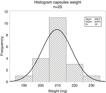

Fig. 20.1
Histogram of capsule weights (n = 20)
When the number of observations is increased and the class interval size is reduced (Fig. 20.2 Histogram of a large sample or population), the histogram appears to become smoother. At an infinitely large number of observations and an infinitesimally small class interval size a probability density curve appears. Well known is the so called Gaussian or normal distribution, that applies to numerous situations in science e.g. the distribution of measurement errors, of genetic variation or, generally, of the sum of a large number of random variates, see Fig. 20.2. Other distributions are the binomial distribution and the Poisson distribution.
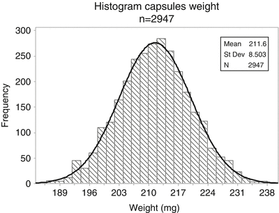

Fig. 20.2
Histogram of a large sample or population
A quantitative measure of variation is the range, i.e. the difference between the highest and the lowest value (if existing) in the population or in the sample. The significance of this parameter is limited because only two elements in the sample determine the degree of variation making it unreliable.
A more reliable measure of the variation of a population distribution is the standard deviation (σ):
![$$ \upsigma =\surd \Big[{\displaystyle {\sum}_{i=1}^n{\left(\upmu - {x}_i\right)}^2/\mathrm{n}\Big]} $$](/wp-content/uploads/2017/01/A315000_1_En_20_Chapter_Equ3.gif)
i.e. the square root of the mean of the squared deviations of the population values (xi) to the population mean (μ).
![$$ \upsigma =\surd \Big[{\displaystyle {\sum}_{i=1}^n{\left(\upmu - {x}_i\right)}^2/\mathrm{n}\Big]} $$](/wp-content/uploads/2017/01/A315000_1_En_20_Chapter_Equ3.gif)
(20.2)
Equation 20.2 is appropriate when the n elements form a population, e.g. a batch consisting of 30 divided powders. If the n elements form a sample taken from a larger population then Eq. 20.3 applies.
The standard deviation of the sample (s) when the population mean (μ) and standard deviation of the population (σ) are unknown is computed as:
![$$ \mathrm{s} = \surd \Big[{\displaystyle {\sum}_{i=1}^n{\left(\mathrm{m}-{x}_i\right)}^2/\left(\mathrm{n} - 1\right)\Big]} $$](/wp-content/uploads/2017/01/A315000_1_En_20_Chapter_Equ4.gif)
where m is defined in Eq. 20.1a and division is by n − 1, the number of degrees of freedom.
![$$ \mathrm{s} = \surd \Big[{\displaystyle {\sum}_{i=1}^n{\left(\mathrm{m}-{x}_i\right)}^2/\left(\mathrm{n} - 1\right)\Big]} $$](/wp-content/uploads/2017/01/A315000_1_En_20_Chapter_Equ4.gif)
(20.3)
The sample variance (s2) is an unbiased estimate (see Sect. 20.2.1) of the population variance (σ2), because it can be proved that for k → ∞:

Note that division in Eq. 20.3 by n instead of by n − 1 produces a biased, too small, estimate of the population variance.

(20.3a)
The population standard deviation of an analysis method will often be estimated from two or more duplicates, i.e. samples with n = 2, taken from different populations:
![$$ \mathrm{s} = \surd \Big[{\displaystyle {\sum}_{i=1}^k{d}_i^2/2\mathrm{k}\Big]} $$](/wp-content/uploads/2017/01/A315000_1_En_20_Chapter_Equ6-1.gif)
where di = the difference of two duplicate values, i = 1, 2, …, k; k = the number of duplicates; s has k degrees of freedom, since each independent duplicate attributes one (2 − 1) degree of freedom.
![$$ \mathrm{s} = \surd \Big[{\displaystyle {\sum}_{i=1}^k{d}_i^2/2\mathrm{k}\Big]} $$](/wp-content/uploads/2017/01/A315000_1_En_20_Chapter_Equ6-1.gif)
(20.4)
The standard deviation has the same dimension as the mean to which it relates, e.g. 20 capsules, weighing 215.2 mg on the average may have a standard deviation amounting to 8.4 mg.
To compare standard deviations the relative standard deviation (rsd) or coefficient of variation, may be useful:

The relative standard deviation is dimensionless and is expressed in proportions or percentages.

(20.5)
The standard deviation of a sample (Eq. 20.3) is an estimate of the standard deviation of the corresponding population distribution.
Quite a different notion is the distribution of a sample statistic such as the sample mean or the sample standard deviation. For instance samples taken from a population with parameters μ and σ2 have themselves a distribution with mean μ and variance  where n is the sample size. The square root of σ m 2 is often called the standard error of the mean or SEM:

If σ is unknown, it can be replaced by s, the sample standard deviation (Eq. 20.3). The equation expresses the well-known fact, that the sample mean becomes more precise with the reciprocal of the sample size. This ‘law of the large numbers’ implies that for obvious reasons the standard error of the mean becomes zero if the sample size approaches infinity.
 where n is the sample size. The square root of σ m 2 is often called the standard error of the mean or SEM:
(20.6)
More generally the standard deviation of any statistic is called a standard error of that statistic being a measure of the imprecision with which the statistic is determined.
20.2.3 Random and Systematic Errors
Both random and systematic deviations may refer to the actual properties of the elements in a population, but frequently also to errors occurring during the manufacturing process or errors occurring in the QC laboratory. The weights of individual suppositories in a lot will exhibit random variation around the average, and when the wrong mold is used, the weights are systematically too high or too low.
Another source of random or systematic deviations may be the measurement process itself. When running a series of six assays of the active substance in an oral solution, the observed variability solely is caused by the analysis, provided the active substance is completely dissolved in the solution and the solution is homogeneous.
Uncorrected background absorption in a spectrophotometric UV–determination is an example of a systematic error, caused by the measuring process. However, background absorption may also be caused by components from the matrix in an unpredictable way and may then be random.
The effect of random deviations on the determination of the population mean can be eliminated by increasing the number of samples or the sample size. As a result the observed mean approaches more and more the true mean of the population. The effect of systematic deviations is independent of the number of samples or the sample size, and can only be eliminated by taking away the cause (the correct suppository mold) or in case of the UV-determination by correction for background absorption.
20.3 Confidence Intervals
20.3.1 Probability and Confidence Intervals
When the population distribution is known, for example X is normally distributed with mean μ and variance σ2, we may calculate the probability of X being equal to or larger than x (X ≥ x). We use that principle for e.g. process control by control charts. The production process has known targets for μ and σ2 and when an uncommon value of variable X ≥ x is observed, the production process should be adjusted.
Very often the population is only known or assumed to have a normal (or other type of) distribution and we want to estimate the unknown values of μ and σ2. To do that, we take a sample from the population and determine the sample mean, m, and the variance of the sample, s2 (with n − 1 degrees of freedom). Both are unbiased estimates (see Sect. 20.2.1) of the corresponding population parameters μ and σ2, meaning that, if we repeat the determination numerous times, the mean of all sample means approaches μ and, equally, the mean of all sample variances approaches the true value σ2.
In practice, only one or a few determinations are performed leaving us with uncertainty in the estimates of the population parameters.
A confidence interval is then the interval of values of m (or s2), that comprises the true value of μ (or σ2) in, say, 95 of 100 cases. The latter is called the confidence level and can be varied at will. In other words when we repeat the determination a large number of times, we are sure that, in about 95 % of the repetitions the true value of μ (or σ2) is captured by the confidence interval.
An example is the assay of dexamethasone capsules using a sample of six capsules with observed mean m = 97.4 % and standard deviation s = 4.0 %.
The 95 % confidence interval is (for details see Sect. 20.3.2):

where t5,0.025 (= 2.57) is the value of the t-distribution with 6 − 1 = 5 degrees of freedom and an upper tail probability of 2.5 % and t5,0.975 (= −2.57) the lower tail probability of 97.5 %.

(20.7)
The lower limit of the 95 % confidence interval is 93.2 % and the upper limit equals 101.5 %.
Mark that, when the determination is repeated again and again, the confidence interval will change each time, because calculation of the upper and lower limits requires the values of the sample mean and standard deviation whose values will vary from sample to sample.
The result should be interpreted carefully. We have only an estimate of the value of the population mean and we know that each time the limits of the confidence intervals change.
However, we can be confident that upon repeating the assay sufficiently often, we approach the true value of μ more and more and that μ is within the calculated confidence intervals in say 95 % of the cases.
Confidence intervals provide a method of stating both how close the value of a statistic (e.g. the sample mean) is likely to be to the value of a parameter (μ) and the probability of its being that close. Mark that the confidence level 95 % is not the probability that the statistic is equal to the population parameter. It is a statement about our confidence in the method we use to estimate the true value and to how close we can come to it. Also the population parameter, μ, is a fixed value and has no probability distribution.
The normal distribution is known as a bell shaped curve of x against its probability density, f(x), and is characterised by two parameters: the average, μ, and the variance, σ2, see Fig. 20.3. The area under the probability density curve, f(x), between two values, say x1 and x2, is equal to the chance of finding a value between x1 and x2, P(x1 < X < x2), in the population. If x1 = − ∞ and x2 = + ∞ the area is equal to 1.
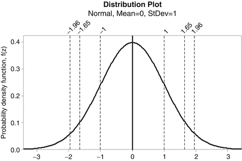

Fig. 20.3
Probability density function of the standard normal distribution with 

Note:
68 % of the elements are between μ + σ and μ – σ
90 % of the elements are between μ + 1.65σ and μ – 1.65σ
95 % of the elements are between μ + 1.96σ and μ – 1.96σ
If μ = 0 and σ2 = 1 the normal distribution is called the standard normal distribution. Any normally distributed variable, X, can be transformed to the variable Z that has the standard normal distribution through equation:

Z can easily be seen to have the standard normal distribution with μ = 0 and σ2 = 1.

(20.8)
Values of P (z < Z < ∞) of the standard normal distribution are called upper tail (or one-sided) probabilities. Since the normal distribution is symmetric, the lower tail probabilities P (−∞ < Z < z) have the same values as their upper tail equivalents. They are usually tabulated as a function of z in books and on internet sites, see Table 20.1 for a small sample.
Table 20.1
Upper tailed probabilities of the standard normal distribution. More extensive tables for the standard normal distribution can be found in books and on the internet
z | P (z < Z < ∞) |
|---|---|
0.50 | .3085 |
1.00 | .1587 |
1.50 | .0668 |
1.645 | .050 |
1.96 | .025 |
2.00 | .023 |
2.576 | .005 |
3.00 | .0013 |
Thus from Table 20.1 it can be read that for the standard normal distribution a proportion of 1 − 2 × 0.1587 = 0.683 or 68.3 % of the population is found between plus and minus one standard deviation, σ, from the mean μ. The abscissa of the standard normal distribution is calibrated in standard deviation units, see Fig. 20.3.
Also for the standard normal distribution 2.5 % of the elements is larger than 1.96, 2.5 % of the elements is smaller than −1.96 and the remaining 95 % is between −1.96 and +1.96. Back transforming using Eq. 20.9 to the corresponding normal distribution with parameters μ and σ2, 2.5 % of the elements is larger than μ + 1.96 σ, 2.5 % of the elements is smaller than μ − 1.96 σ and 95 % of the elements is between μ − 1.96 σ and μ + 1.96 σ, i.e.

comprises 95 % of the values of X, when X is normally distributed with parameters μ and σ2, see also Fig. 20.3. So, if μ = 100 and σ = 5, X is between 100 − 1.96 × 5 = 90.2 and 100 + 1.96 × 5 = 109.8.

(20.9)
20.3.2 Confidence Interval of μ if the Standard Deviation of the Population is Known
Equation 20.9 can be converted to:

Equation 20.10 is one version of the confidence interval defined in the introduction of this section. The real value of μ will be located in 95 out of 100 cases in the confidence interval. This is the double-sided 95 % confidence interval of μ, the right-tailed form of the 95 % confidence interval is:

which says that the real value of μ will in 95 out of 100 cases be smaller than x + 1.645 σ. The value z0.95 = 1.645 corresponds to the upper tail probability of 0.05 in Table 20.1. The left tail confidence interval is analogous to the upper tail interval.

(20.10)

(20.11)
The sampling distribution of the mean of n independent observations has mean μ and standard error equal to  Eq. 20.6.
 Eq. 20.6.
Assuming normal distribution of the sample mean, m, we obtain for the 100(1−α) % confidence interval:

where α/2 is the upper tail probability and zα/2 can be found in Table 20.1. For instance zα/2 = 1.96 if α/2 = 0.025, giving the 100(1 – 0.05) % = 95 % confidence interval.

(20.12)
The width of the confidence interval is inversely proportional to √n, which implies that if the sample size increases, the sample mean is a more precise, but not necessarily a more accurate estimate of the population mean, see Fig. 20.4 Confidence intervals (95 % confidence level).
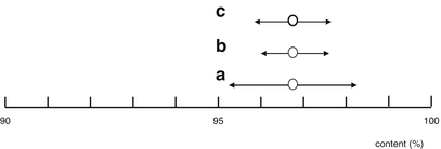

Fig. 20.4
Confidence intervals (95 % confidence level).
(a): μ = 96.8, σ = 0.8, n = 1; 95 % confidence interval = 96.8 ± 1.6.
(b): μ = 96.8, σ = 0.8, n = 4; 95 % confidence interval = 96.8 ± 0.8.
(c): μ = 96.8, s = 0.6, n = 4; 95 % confidence interval = 96.8 ± 0.95
Worked Example: See Fig. 20.4 sub a
A control laboratory for pharmacy preparations knows by experience that the standard deviation of the determination of noscapine hydrochloride in an oral solution by means of U.V.-measurement equals 0.8 %.
When the outcome is 96.8 %, the true content of the oral solution is with 95 % confidence 96.8 ± 1.96 × 0.8, i.e. between 98.4 % and 95.2 %. Or, the true content is with 95 % confidence above 96.8 + 1.645 × 0.8 = 98.1 % (down to 0 %, which is in this example of course unrealistic).
Note: when calculating the confidence interval please check that the standard deviation, and not the relative standard deviation is used.
The choice of the confidence level is arbitrary. We could have chosen 99 % instead of 95 % confidence by replacing 1.96 with 2.58. A wider interval will have a higher probability of including μ, but the statement loses precision.
Worked Example: See Fig. 20.4 sub b
The determination of noscapine hydrochloride in the oral solution, see previous example, will be quadruplicated. The mean of the four observations is 96.8 %.
The true content of the oral solution with 95 % confidence is between 96.8 ± 1.96 × 0.8/√4 i.e. between 96.0 % and 97.6 %.
20.3.3 Confidence Interval of μ if the Standard Deviation of the Population is not Known
If the standard deviation of the population (σ) is unknown, confidence statements have to be based on the sample standard deviation, s. In the equation for the confidence interval (Eq. 20.12) the value zα/2 is replaced by the corresponding value tν,α/2 of Student’s t-distribution. The result is:

The value of tν,α/2 depends on the number of degrees of freedom (ν) and the desired confidence level, (1 − α). Student’s t-distribution and t-test have been invented by Gosset (his pen name was Student) as early as 1908.

(20.13)
The number of degrees of freedom is n − 1, if the sample standard deviation, s, is obtained from one sample. It may eventually be obtained from a series of K samples by pooling si, i = 1, 2, …, K with degrees of freedom νi, i = 1, 2, …, K:

Values of t for different numbers of degrees of freedom and upper tail probabilities can be looked up in a t-distribution table such as Table 20.2. More extensive tables can be consulted in books and on the internet.

(20.14)
Table 20.2
Values of tν, α/2 for selected upper tailed probabilities, α/2, and degrees of freedom, ν, of the t-distribution
α/2 | Degrees of freedom | |||||
|---|---|---|---|---|---|---|
2 | 3 | 5 | 10 | 20 | ∞ | |
.50 | 0.000 | 0.000 | 0.000 | 0.000 | 0.000 | 0.000 |
.30 | 0.617 | 0.584 | 0.559 | 0.542 | 0.533 | 0.525 |
.20 | 1.061 | 0.978 | 0.920 | 0.879 | 0.860 | 0.839 |
.10 | 1.886 | 1.638 | 1.476 | 1.372 | 1.325 | 1.279 |
.05 | 2.920 | 2.353 | 2.015 | 1.812 | 1.725 | 1.645 |
.025 | 4.303 | 3.182 | 2.571 | 2.228 | 2.086 | 1.960 |
.010 | 6.965 | 4.541 | 3.365 | 2.764 | 2.528 | 2.327 |
.005 | 9.925 | 5.841 | 4.032 | 3.169 | 2.845 | 2.576 |
Worked Example: See Fig. 20.4 sub c
The assay of noscapine hydrochloride in the oral solution, see previous example, has been run in fourfold but now the standard deviation of the population is unknown and estimated by the sample standard deviation s = 0.6 with ν = 4 − 1 = 3 degrees of freedom. The sample mean is 96.8 %. The upper tailed α/2 = 0.025 t-value with ν = 3 is t3, 0.025 = 3.182.
According to Eq. 20.13 the two-sided 95 % confidence interval of the true content, μ, is 96.8 – t3, 0.025 × s/√4 < μ < 96.8 + t3, 0.025 × s/√4 = 96.8 − 3.18 × 0.6/2 < 96.8 + 3.182 × 0.6/2 = 95.8 < μ < 97.8.
20.3.4 Confidence Interval of the Variance σ2, and the Standard Deviation σ
The sample variance, s2, is an unbiased estimate (see Sect. 20.2.1) of the population variance, σ2, with ν degrees of freedom. The statistic νs2 has the chi-square distribution with ν degrees of freedom. The 100(1–α) % two-sided confidence interval is:


