A Community Screening Programs

In a population with a low prevalence of a particular disease, most of the positive results in a screening program for the disease likely would be falsely positive (see Chapter 7). Although this fact does not automatically invalidate a screening program, it raises some concerns about cost-effectiveness, which can be explored using Bayes theorem.

A program employing the tuberculin tine test to screen children for tuberculosis (TB) is discussed as an example (based on actual experience).³ This test uses small amounts of tuberculin antigen on the tips of tiny prongs called tines. The tines pierce the skin on the forearm and leave some antigen behind. The skin is examined 48 hours later, and the presence of an inflammatory reaction in the area where the tines entered is considered a positive result. If the sensitivity and specificity of the test and the prevalence of TB in the community are known, Bayes theorem can be used to predict what proportion of the children with positive test results will have true-positive results (i.e., will actually be infected with Mycobacterium tuberculosis).

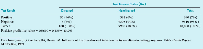
Box 8-1 shows how the calculations are made. Suppose a test has a sensitivity of 96% and a specificity of 94%. If the prevalence of TB in the community is 1%, only 13.9% of those with a positive test result would be likely to be infected with TB. Clinicians involved in community health programs can quickly develop a table that lists different levels of test sensitivity, test specificity, and disease prevalence that shows how these levels affect the proportion of positive results that are likely to be true-positive results. Although this calculation is fairly straightforward and extremely useful, it is not used often in the early stages of planning for screening programs. Before a new test is used, particularly for screening a large population, it is best to apply the test’s sensitivity and specificity to the anticipated prevalence of the condition in the population. This helps avoid awkward surprises and is useful in the planning of appropriate follow-up for test-positive individuals. If the primary concern is simply to determine the overall performance of a test, however, likelihood ratios, which are independent of prevalence, are recommended (see Chapter 7).

Box 8-1 Use of Bayes Theorem or 2 × 2 Table to Determine Positive Predictive Value of Hypothetical Tuberculin Screening Program

Part 1 Beginning Data

Sensitivity of tuberculin tine test	= 96%	= 0.96
False-negative error rate of test	= 4%	= 0.04
Specificity of test	= 94%	= 0.94
False-positive error rate of test	= 6%	= 0.06
Prevalence of tuberculosis in community	= 1%	= 0.01

Data from Jekel JF, Greenberg RA, Drake BM: Influence of the prevalence of infection on tuberculin skin testing programs. Public Health Reports 84:883–886, 1969.

Part 2 Use of Bayes Theorem

Part 3 Use of 2 × 2 Table, with Numbers Based on Study of 10,000 Persons

Positive predictive value = 96/690 = 0.139 = 13.9%

There is another important point to keep in mind when planning community screening programs. The first time a previously unscreened population is screened, a considerable number of cases of disease may be found, but a repeat screening program soon afterward may find relatively few cases of new disease. This is because the first screening would detect cases that had their onset over many years (prevalent cases), whereas the second screening primarily would detect cases that had their onset during the interval since the last screening (incident cases).

B Individual Patient Care

Suppose a clinician is uncertain about a patient’s diagnosis, obtains a test result for a certain disease, and the test is positive. Even if the clinician knows the sensitivity and specificity of the test, this does not solve the problem, because to calculate the positive predictive value, whether using Bayes theorem or a 2 × 2 table (e.g., Table 7-1), it is necessary to know the prevalence of the disease. In a clinical setting, the prevalence can be considered the expected prevalence in the population of which the patient is part. The actual prevalence is usually unknown, but often a reasonable estimate can be made.

For example, a clinician in a general medical clinic sees a male patient who complains of easy fatigability and has a history of kidney stones, but no other symptoms or signs of parathyroid disease on physical examination. The clinician considers the probability of hyperparathyroidism and decides that it is low, perhaps 2% (reflecting that in 100 similar patients, probably only 2 of them would have the disease). This probability is called the prior probability, reflecting that it is estimated before the performance of laboratory tests and is based on the estimated prevalence of a particular disease among patients with similar signs and symptoms. Although the clinician believes that the probability of hyperparathyroidism is low, he or she orders a serum calcium test to “rule out” the diagnosis. To the clinician’s surprise, the results of the test come back positive, with an elevated level of 12.2 mg/dL. The clinician could order more tests for parathyroid disease, but even here, some test results might come back positive and some negative.

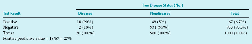
Under the circumstances, Bayes theorem could be used to help interpret the positive test. A second estimate of disease probability in this patient could be calculated. It is called the posterior probability, reflecting that it is made after the test results are known. Calculation of the posterior probability is based on the sensitivity and specificity of the test that was performed and on the prior probability of disease before the test was performed, which in this case was 2%. Suppose the serum calcium test had 90% sensitivity and 95% specificity (which implies it had a false-positive error rate of 5%; specificity + false-positive error rate = 100%). When this information is used in the Bayes equation, as shown in Box 8-2, the result is a posterior probability of 27%. This means that the patient is now in a group of patients with a substantial possibility, but still far from certainty, of parathyroid disease. In Box 8-2, the result is the same (i.e., 27%) when a 2 × 2 table is used. This is true because, as discussed previously, the probability based on the Bayes theorem is identical to the positive predictive value.

Box 8-2 Use of Bayes Theorem or 2 × 2 Table to Determine Posterior Probability and Positive Predictive Value in Clinical Setting (Hypothetical Data)

Part 1 Beginning Data (Before Performing First Test)

Sensitivity of first test	= 90%	= 0.90
Specificity of first test	= 95%	= 0.95
Prior probability of disease	= 2%	= 0.02

Part 2 Use of Bayes Theorem to Calculate First Posterior Probability

Part 3 Use of a 2 × 2 Table to Calculate First Positive Predictive Value

Positive predictive value = 18/67 = 27%

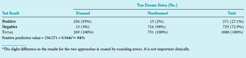
In light of the 27% posterior probability, the clinician decides to order a serum parathyroid hormone concentration test with simultaneous measurement of serum calcium, even though this test is expensive. If the parathyroid hormone test had a sensitivity of 95% and a specificity of 98%, and the results turned out to be positive, the Bayes theorem could be used again to calculate the probability of parathyroid disease in this patient. This time, however, the posterior probability for the first test (27%) would be used as the prior probability for the second test. The result of the calculation, as shown in Box 8-3, is a new probability of 94%. The patient likely does have hyperparathyroidism, although lack of true, numerical certainty even at this stage is noteworthy.

Box 8-3 Use of Bayes Theorem or 2 × 2 Table to Determine Second Posterior Probability and Second Positive Predictive Value in Clinical Setting

Part 1 Beginning Data (Before Performing the Second Test)

Sensitivity of second test	= 95%	= 0.95
Specificity of second test	= 98%	= 0.98
Prior probability of disease (see Box 8-2)	= 27%	= 0.27

Part 2 Use of Bayes Theorem to Calculate First Posterior Probability

Part 3 Use of 2 × 2 Table to Calculate First Positive Predictive Value

Positive predictive value = 256/271 = 0.9446*= 94%

^*The slight difference in the results for the two approaches is caused by rounding errors. It is not important clinically.

Why did the posterior probability increase so much the second time? One reason was that the prior probability was considerably higher in the second calculation than in the first (27% versus 2%), based on the first test yielding positive results. Another reason was that the specificity of the second test was assumed to be quite high (98%), which greatly reduced the false-positive error rate and increased the PPV. A highly specific test is useful for “ruling in” disease, which in essence is what has happened here.

C Influence of the Sequence of Testing

With an increasing number of diagnostic tests available in clinical medicine, the clinician now needs to consider whether to do many tests simultaneously or to do them sequentially. As outlined in Chapter 7, tests used to “rule out” a diagnosis should have a high degree of sensitivity, whereas tests used to “rule in” a diagnosis should have a high degree of specificity (see Box 7-1). The sequential approach is best done as follows:

Compared with the simultaneous approach, the sequential approach to testing is more conservative and is more economical in the care of outpatients. The sequential approach may increase the length of stay for a hospitalized patient, however, so the cost implications may be unclear.

The sequence of testing may have implications for the overall accuracy. If multiple diagnostic tests are performed at the same time, the natural tendency is to ignore the negative results, while seriously considering the positive results. This approach to establishing a diagnosis may not be ideal, however. Even if the tests are performed simultaneously, it is probably best to consider first the results of the most sensitive test. If a negative result is reported for that test, the result is probably a true-negative one (the patient probably does not have the disease). Why? Highly sensitive tests are reliably positive when disease is present and tend to deliver negative results only when disease is truly absent. Simultaneous testing may produce conflicting results, but a careful consideration of each test’s result in light of the test’s sensitivity and specificity should improve the chances of making the correct diagnosis.