However, because of the nature of the syndrome, we are at liberty to do the study a little differently than the usual approach. Assuming that committees meet only every week or two, and that the pain subsides in hours, then we have a suitable washout period, so that we can use each subject again every 2 weeks.

So, instead of randomly assigning individuals to take one of the analgesics, we can actually ask each person to take all of the analgesics, in turn, separated by 2 weeks between meetings, and suitably blinded, of course. It’s just a generalization of the paired t-test, in which each person was assessed twice and the difference between the two occasions calculated. Now we will deal with multiple assessments,³ but the basic idea of each subject becoming his or her own control holds true. This amounts to directly assessing the variance owing to systematic differences between subjects, leaving less variance in the error term (if all goes well).

As a design aside, in order to ensure that order effects are not confounded with treatment effects, we would likely randomize the order of treatment so that ⅓ got Entrophen first, ⅓ got Tylenol first, and ⅓ got Motrin first. If we didn’t do that, and all the people are in a long, natural healing course as they grow tolerant of the irritant and learn to tune him out, it might appear that the last medication worked the best. Down the road, we’ll talk about how to analyse the data to see if there are order effects.

REPEATED-MEASURES ANOVA (ONE FACTOR)

The design we’re talking about is called a repeated-measures ANOVA for, we hope, fairly obvious reasons. The data may look something like Table 11–1.

Conceptually, we are in the same situation as we were when we made the transition from an unpaired t-test to one-way ANOVA. In the first instance, we just want to determine whether there is any overall difference among the analgesics; it is of secondary importance to figure out whether 1 differs from 2, 2 from 3, and so on. The approach, just like the other ANOVAs we have encountered to date, is to examine the sources of variance. The important distinction in this design, however, is that there are repeated observations on each subject so that we can separate out subject variance from error variance. In the ordinary ANOVA designs, subjects are assigned at random (hopefully) to different groups, and any differences between subjects in the variable of interest ultimately ends up as error variance in the test of the effect of the grouping factors. Here, however, we can take the average of all the observations on each subject as a best guess at the true value of the variable for each subject. The subject variance is then calculated as the difference among these subject means, and the error variance is determined by the dispersion of individual values around each subject mean.

Looking at it this way, then, there are actually three sources of variance:

TABLE 11–1 Pain relief from various analgesics

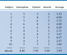
1. Differences among analgesics overall (at the bottom of the columns)
   
2. Differences among subjects in the average rating of improvement (right hand column)
   
3. Error variance—the extent to which an individual value in a cell is not predictable from the margins

If we continue to look at it this way a bit longer, we see that the design is actually a two-way ANOVA, with the individual subjects as one factor and the pain reliever as a second factor. So the cells are now defined by the factors Subject with 10 levels and Drug with 3 levels. There are 30 cells and 30 observations, so there is only one observation per cell. Let’s plow ahead, using exactly the same approach as before.

Starting with the formula:

so the calculation is:

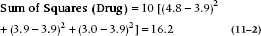
Remember that since this effect doesn’t include Subject, which has 10 levels, we have to multiply the whole ruddy thing by 10. Putting it another way, there are only three terms, so we multiply by 10 to make it come out to 30.

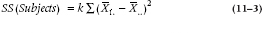
For the Sum of Squares (Subjects), the formula is:

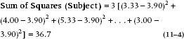
Similarly, since this effect is missing the Drug, with 3 levels, we multiply the sum of squared differences by 3.

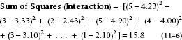
Now, to calculate the interaction term, it is necessary to estimate the expected values in each cell. We went through the logic before, and it results in an expected value for the first few cells as shown in Table 11–2.

So, the interaction sum of squares is:

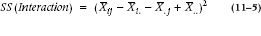
No multiplier is necessary this time since there are already 30 terms.

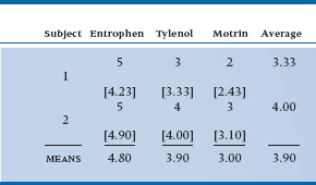
Estimation of degrees of freedom is just like before. For the Drug main effect, there are three data points and one grand mean, so (3 − 1) = 2 degrees of freedom. For the Subject main effect, there are 10 data points and one mean, so (10 − 1) = 9 df. And finally, for the interaction, there are (10 − 1) × (3 − 1) = 18 df. This all totals to 18 + 9 + 2 = 29 df, one less than the total number of data, so we must have got it right.⁴

We can now do the last step and create the Mean Squares and the ANOVA table, as shown in Table 11–3.

Our research hypothesis asks whether there is any significant difference in relief from the various pain relievers. This is simply captured in the main effect of Drug. The error term for this comparison is the Subject × Drug Mean Square, since this reflects the extent to which different subjects respond differently to the different drug types. That is, just as in an ordinary ANOVA, differences between subjects is a measure of error in the estimate of the effect. The only difference is that, since we have multiple measures for each subject, this amounts to a Subject × Drug interaction.

The test of significance, then, is based on the ratio of Mean Square (Drug) to Mean Square (Subject × Drug), and equals 9.22, as shown in the ANOVA table (Table 11–3). This is significant at the .005 level.

As you can see, the Subject term contributes to the total sum of squares, but there’s no F-test associated with it. In most cases where repeated-measures ANOVAs are used, subjects are just “replicates,” as they are in between-subjects ANOVAs. We do use this term, though, in a branch of scale development called Generalizability Theory, when we are trying to determine the different factors that may contribute to the unreliability of a measure (Streiner and Norman, 2014).

One last run through these data, before we go on to bigger and better things. As we indicated at the start, we could have done the experiment in a different way by simply randomly assigning individuals to each of the three analgesic groups. That is, instead of measuring 10 people three times, we could have used 30 people and measured each only once. Let’s pretend, for the moment, that the data from Table 11–1 came from this design. The appropriate analysis would be a simple one-way ANOVA, and the ANOVA table would look like Table 11–4.

Although the total Sum of Squares is the same, the variance owing to subjects and the error variance are now lumped together, leading to a bigger error term for the test of the drug effect, which is now not so highly significant. The reason is that we are no longer able to extract variance owing to systematic differences between subjects, since we have only one observation for each subject.

We have described repeated-measures ANOVA in its simplest form. It is a natural extension of the paired t-test, just as the one-way ANOVA is an extension of the unpaired t-test. In fact, some people call it a one-way repeated-measures ANOVA.

TABLE 11–2 Observed and expected values (in square brackets) for first two subjects

Another parallel holds. Like the paired t-test, repeated-measures ANOVA is able to take account of systematic differences between subjects, which usually leads to more powerful tests. Finally, like the one-way ANOVA, it is the simplest of the class of designs, and the basic method extends naturally to more complex ones.

GENERALIZATION TO INCLUDE OTHER TRIAL FACTORS

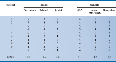
You may have noticed in passing that all the drugs we have used to date were brand names. Here’s a chance to address the age-old question of brand name versus generic and, at the same time, learn a little more about the arcane delights of repeated-measures ANOVA. The strategy we used to go from one-way to two-way ANOVA, and to include a second factor in the design, can be applied to repeated observations, only this time we capture the unsuspecting academics for six meetings, three with brand names (Entro-phen, Tylenol, Motrin) and three with the equivalent generics (ASA, acetaminophen, ibuprofen).⁵ The design is shown in Table 11–5; we have thrown in some additional data.

TABLE 11–3 Analysis of variance summary table

TABLE 11–4 Analysis of variance summary table for an equivalent between-groups design

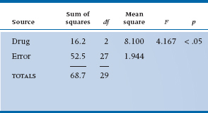
TABLE 11–5 Two-factor repeated-measures design (analgesic type, brand/generic)

The first challenge is to work out all the possible lines in the ANOVA table. To start, there are now two factors: Drug (as before) with three levels, and now Brand/Generic with two levels. These are the two main effects. Again as before, subjects are just replications of the study, unless we’re dealing with Generalizability Theory, and they don’t appear in the table. As we showed in Table 11–5, this means there are 3 × 2 = 6 observations on each subject. We now examine some interactions: Drug × Brand/Generic (whether the differences between drugs are the same for brand names and generics); and several interactions with subjects—Subject × Drug (whether some subjects respond differently to some drug types more than others), Subject × Brand/Generic (whether some subjects show different responses to brands and generics), and Subject × Drug × Brand/Generic (we won’t even try to put this one into words). Again, generalizing from the first example, every Subject × Something interaction is the error term to test the effect, since it amounts to differences in the effect for different people.

TABLE 11–6 Analysis of variance summary table of data in Table 11–5

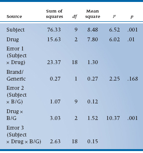
The Sums of Squares are computed using the general strategy of computing differences between individual means and the grand mean for main effects, and differences between individual cell means and their expected value from the marginals for interactions, in each case multiplying by some fudge factor corresponding to the number of levels of the remaining factors. So, for the main effect of Drug, there are three terms in the Sum of Squares, corresponding to the mean of ASA and Entrophen (4.35) subtracted from the grand mean (3.833), the mean of Tylenol and acetaminophen (3.85), and the mean of Motrin and ibuprofen (3.20), all squared up and multiplied by the famous fudge factor, which is now 2 × 10 = 20, to get a result of 60 terms. After the dust settles, we have Table 11–6.

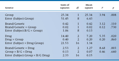
As the table shows, we found an overall main effect of Drug (F = 6.02, df = 2/18, p = .01), but no overall effect of Brand/Generic (F = 2.25, df = 1/9, p = .168). However, we are a bit surprised to see a Drug × Brand/Generic interaction, indicating that the differences between drug classes are different for brands and generics. That shows up when we inspect the table a bit closer and see that, although ASA-based drugs are most effective, the effect is smaller for the generic (4.1 versus 4.8); similarly, ibuprofen is the least effective drug, but the generic is actually a bit more effective than the brand (3.4 versus 3.0). Such are the vagaries of science.

If you want a name for this design, it’s called a two-way repeated-measures ANOVA. Note that we are simply using the same basic strategy to encompass a design where the repeated observations arise from more than one factor.

Between-Subjects and Within-Subjects Factors

Now that we are used to the idea of including more than one repeated factor in the design, we can bring up the heavy artillery and contemplate a world where both repeated observations within each subject, and other factors that group subjects into classes, arise together in the same design. One way to think about the distinction is to class all the factors as either within-subjects or between-subjects. The two factors that we have encountered to date, Drug and Brand/Generic, both occur as repeated observations for each subject in the design and are, therefore, called within-subject factors.

A within-subjects (trial) factor is one in which all levels of the factor are present for each subject; that is, it results in repeated measures.

What would a between-subject factor look like? Well, let’s expand the design one last time. Perhaps we are concerned that ME is prevalent for only some kinds of committees. From personal experience, ME carriers seem to gravitate to administrative committees, which are inevitably burdened with routine decision making necessary to keep the academic ship afloat. Carriers tend to avoid the more creative committees like research-group meetings. Perhaps the severity of ME is lower in research meetings, or the effects are more transient so that relief comes more rapidly.

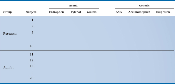
How would we put it to a test? We would use the same design as before, only this time we recruit 10 academics from an administrative committee and 10 different academics from a research group.⁶,⁷ The design would now look like Table 11–7.

We have the same two within-subject factors as before. However, we now have an additional factor, Group (i.e., type of committee), which is different. It can assume only one value for each subject; that is, a particular person can only be a on an administrative committee or a research committee, not both (see note 6), and subjects are grouped under each level of this factor. By extension, this is called a between-subjects or grouping factor.

A between-subjects or grouping factor is one in which each subject is present at only one level of the factor; that is, subjects are grouped under a level of the factor.

As a matter of course, it is usually easier in these repeated-measures designs to put all the between-subjects factors on the left and all the within-subjects factors on the top. This guarantees that the innermost column on the left will be “Subject,” and that each row corresponds to all the measurements on one subject—in this case, six.

Now, let’s proceed to anticipate what the ANOVA table might look like. We won’t do it, since, as yet, there are no data in the boxes.⁸ To begin, there are four main effects: Group (Do folks on research committees get more relief from ME pain than those on administrative committees?) and Subject (Do some people get more or less relief than others?) from the left column; and Drug (Do all drugs give the same relief?) and Brand/Generic (Do brand name drugs give the same relief as generic drugs?) from the top rows. There are also some two-way interactions—Group × Brand/Generic, Group × Drug, and as before Drug × Brand/Generic. There are also several interactions with Subject, which will find their way into the assorted error terms.

The one interaction with Subject that is missing is the Subject × Group term. Since each patient is on either an administrative or a research committee, not both, we can’t estimate this interaction. This is just another way of saying that Group is a between-subjects factor.

TABLE 11–7 Experimental design for inclusion of between- and within-subject factors

A more general way of describing this idea is to speak of crossed and nested factors, which we first came across in Chapter 9.

Two factors are crossed if each level of one factor occurs at all levels of the other factor. A factor is nested in another factor if each level of the first factor occurs at only one level of the second factor.

What was that again? Well, it’s a lot like between-and within-subjects factors. Since Group is a between-subjects factor, each subject can be in either the administrative category or the research category, not both; so, Subject is nested within Group. However, since both Group and Subject occur at all levels of Drug and Brand/Generic (each subject has an observation at all levels of Drug and all levels of Brand/Generic), we say that Subject and Group are crossed with Drug and Brand/Generic. Finally, for completeness, since we have acetylsalicylic acid as both Brand and Generic, Drug and Brand/Generic are themselves crossed factors. Nested factors are often signified with a colon (:) in the ANOVA summary table, so we would write Subject nested within Group as S:Group. So now the whole “kit and caboodle” appears as Table 11–8.

There are a few things to note. First, as we showed in the previous example, there is not a single error term; there are error terms for each main effect and its interaction. For the between-subjects or Group factors, the error term is always Subject: Group, the main effect of subjects. For all the repeated measures, the error terms amount to the associated interaction with Subjects. Second, the ANOVA, although complicated, still obeys some of our fundamental rules: (1) the degrees of freedom add up to one less than the number of data points; (2) the Sums of Squares for individual terms could be summed to yield a Total Sum of Squares; (3) Mean Squares and F-ratios are calculated just as before, except that the correct error term must be used (by the computer of course); and (4) the degrees of freedom for numerator and denominator of the F-ratio must use the right degrees of freedom (but, again, the computer takes care of all this).

In the end, we are simply partitioning variance across multiple factors in order to (1) investigate the possible effects and interactions, and (2) reduce the corresponding error terms and, thereby, increase the power of the test. In particular, one explicit factor in all repeated-measures designs is Subject, so that any variance owing to systematic differences between subjects can be removed and the power of other tests correspondingly increased.

We need not stop here of course. We are limited in the number of factors only by the number of degrees of freedom. In particular, at the outset, we indicated that as good researchers, we should vary the order in which subjects get the different drugs. There’s an easy way to do this and to ensure that it all balances out in the end. It’s called a Latin Square and it is performed as follows. Pick some order—for the sake of argument, Entrophen → Tylenol → Motrin. Now just move everything to the right and rotate the last one to the beginning: Motrin → Entrophen → Tylenol. Do it one last time: Tylenol → Motrin → Entrophen. This exhausts the possibilities. Now ensure that ⅓ of the subjects gets the first sequence, ⅓ the second, and ⅓ the last. If we do this, then we have created a second between-subjects factor. If there is an order effect, it will be apparent and will show up as an Order × Drug interaction.

Finally, let us take a minute to try to convince you that there really is a grand unity to the whole thing. We could have analysed the Group effect differently. We could have said to ourselves, “Ah heck, at the end of the day, we’ve got a bunch of data on 20 folks in two groups. Let’s just average it and do a t-test.” The numerator of the t-test would involve the difference between the overall means for all the data in the administrative and research groups, the same data that are going into the Group main effect. The denominator of the t-test would involve differences between the subject means, the same data that went into the Subject main effect. The resulting t-test would be just the square root of the Group main effect, believe it or not.⁹

TABLE 11–8 Analysis of variance summary for three-factor ANOVA

B/G = Brand/Generic.

Other Applications of Repeated-Measures ANOVA

Repeated-measures ANOVA is a very useful strategy to look at the effects of interventions in situations in which the same person can receive multiple treatments. Any time that a washout period is feasible, then the repeated-measures ANOVA design acts as a generalized crossover study. It also can work with repeated observations at the same time, for example, patch tests for suntan lotions.

However, it has many other applications. Basically, it can be used any time there are repeated measurements on the same set of individuals.¹⁰ One situation in which this occurs is when there are sequential measurements over time, as subjects are followed up for days, weeks, or months. If we did a trial with two groups in which we made repeated observations, we would likely analyze the data with a two-factor repeated-measures ANOVA, with treatment/control as a between-subjects factor and time as a within-subjects factor.¹¹ As we will see in Chapter 17, this is one of several ways to approach the general issue of measuring change.

Another place where we use repeated-measures ANOVA a lot is in measurement studies. When you look at reliability or agreement, whether you use an intraclass correlation or Cohen’s kappa, the starting point is a repeated-measures ANOVA. Interestingly, measurement folks, whose passion is differentiating among people, are really mainly interested in all the things we called “error.”

Finally, repeated-measures designs are one special case of factorial designs and, like factorial designs, the number of possible designs is limited only by imagination and resources.

REPEATED-MEASURES ANOVA AND RELIABILITY OF MEASUREMENT

Repeated-measures ANOVA has one other very useful application—to compute variance components for use in studies of agreement. For example, if we go back to Table 11–1, it is evident that some folks, such as Patient 6, get better relief across the board than others, such as Patient 10. If we turn things around and use the data as a measure of individual susceptibility to pain relief, then we can start to ask whether the measure can reliably distinguish between those who get a lot of relief and those who get a little.

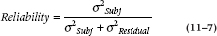
Reliability is usually assessed by the Reliability Coefficient,¹² which is defined as the proportion of variance in the scores related to true variance between the objects of measurement—in this case, patients. The formal definition looks like:

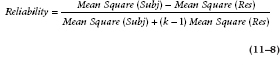
Conveniently, we have the makings of a reliability coefficient in the ANOVA (Table 11–3). Subject variance is directly related to the Mean Square (Subject), and error variance is related to Mean Square (Subject × Drug). Because of the relationship between variances and mean squares, this can be transformed into a computational formula involving Mean Squares. Note that the Mean Square (Residual) is from the Subject × Drug term:

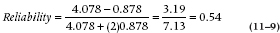
In the present example, then, the reliability is equal to:

The coefficient is called an Intraclass Correlation Coefficient (ICC), since all observations are from the same variable or class; this distinguishes it from the Pearson correlation that has observations from different variables. Fisher called this the “interclass correlation.” It ranges from 0 (no systematic difference between subjects) to 1 (all the variance in scores is due to systematic differences between subjects).

ASSUMPTIONS AND LIMITATIONS OF COMPLEX ANOVA DESIGNS

Are there no costs incurred in this exercise? Of course there are. Nothing comes free, except to selected dictators, capitalists, warlords, and other unscrupulous types. First, just as the case for two-way ANOVA and all other parametric tests, there is the assumption that the data are at least interval level and are normally distributed. We also demand homoscedasticity—a lovely word meaning equal variances. However, we have discussed in Chapter 6 the extent to which the tests are robust to the violation of these assumptions and, as you recall (or we recall), the Central Limit Theorem indicates that for sample sizes over 10 to 20, the normality assumption is unnecessary.¹³ Repeated-measures ANOVA, like all factorial ANOVA designs, imposes one additional constraint; the designs must be balanced or nearly so; this was discussed in Chapter 9. The good news is that, as long as the design is balanced, the ANOVA is robust with respect to assumptions about distributions.

Are there any more limitations? Indeed there are. There are two reasons why one must not continue to add factors into a design at random. First, unless these factors are designed into the study from the outset, they will likely result in imbalance, and we already indicated where that slippery slope leads. Second, there is a law of diminishing returns. Each factor you add, even if you have only two levels of the factor, costs one degree of freedom for the main effect and each interaction. If there are more than two levels, the dfs escalate. Unless the factor is accounting for useful variance, the paradoxical situation can arise that even though the factor carries away some of the Error Sum of Squares, the Error Mean Square term for other analyses actually increases, because the degrees of freedom have been reduced more than the Sum of Squares as a result of the addition of the factor. The upshot is that the mean square—which enters into the statistical test—actually goes up.

Nevertheless, despite the constraints imposed by the addition of more than one factor into a design, the power of analysis and interpretation obtained from factorial and repeated-measures ANOVA is often remarkable, and has added tremendously to the versatility of experimental research.

SAMPLE SIZE ESTIMATION

For all sorts of reasons, there is no exact formula to calculate sample size for two- or three-factor repeated-measures designs. If it is a single factor, and has only two levels, then the procedures outlined for the paired t-test in Chapter 10, which are the essence of simplicity, are appropriate. However, anything more complicated forces us to estimate in advance (1) what might be the appropriate change within subjects, and then, (2) the approximate interaction between subjects and this effect. The last grant writer who went for such long shots jumped off a building in the Crash of ’29.

The best strategy to survive the vagaries of reviewers is to take an approximate approach. Pick the one effect you really care about, which, hopefully, is a main effect with two levels, and use an approximate calculation based on the paired t-test. It still requires a bit of imagination to come up with the error term, but it’s not impossible.

The only exception to this approach is, unfortunately, fairly common: when the effect of concern is a two-way interaction. Here, an even more sweeping approximation is needed. Again we convert this to a pairwise comparison, and then go back to the paired t-test.

REPORTING GUIDELINES

This will be short, because they’re exactly the same as for factorial ANOVA (Chapter 9). Just be sure you’re reporting the df for the correct error term for all those within-subject effects.

SUMMARY

We have considered a number of extensions to the paired t-test, all described as repeated-measures designs. They amount to variations on factorial ANOVA methods, with Subjects as an explicit factor in the design.

EXERCISES

1. For the following designs, name the factor equivalent to “subjects,” then name the between-subjects and within-subjects factors.

a. Thirty spondylitis patients are treated by chiropractors on a weekly basis for 12 weeks. After each treatment, range of motion of the SI joint is measured.

b. Twelve patients suffering from chronic headaches are treated by three different headache medications. At the onset of a headache, each patient selects either a red, white, or blue pill, which he or she selects by throwing a dart at a Union Jack on the basement wall. An hour later, the patient rates the pain on a 10-point scale. This continues until the patient has treated 6 headaches with each color of pill, for a total of 18 headaches per patient.

c. Twelve patients suffering from chronic headaches are treated by three different headache medications. Each patient is randomly assigned to be treated by red, white, or blue pills by the attending physician throwing a dart at a Stars and Stripes on the clinic wall. An hour after the onset of each headache, the patient rates the pain on a 10-point scale. This continues until the patient has treated six headaches.

d. Histologic slides of lymph gland biopsies are judged by pathologists on a 5-point scale for likelihood of cancer. There are 20 slides in total. Each slide is rated by 6 pathologists.

e. Histologic slides of lymph gland biopsies are judged by pathologists on a 5-point scale for likelihood of cancer. There are 20 slides in total. Each slide is rated by 6 pathologists, at 3 levels of experience—2 first-year residents, 2 final-year residents, and 2 pathologists.

f. Histologic slides of lymph gland biopsies are judged by pathologists on a 5-point scale for likelihood of cancer. There are 20 slides in total, all derived from patients with a minimum of 10 years follow-up. Half the slides were from proven normal patients, and the other 10 were from patients who eventually died of lymphoma (cancer of the lymph glands). Each slide is rated by 6 pathologists, at 3 levels of experience—2 first-year residents, 2 final-year residents, and 2 pathologists.

2. To compare 3 of the NSAIDs for the treatment of rheumatoid arthritis, 45 subjects were divided into 3 groups of 15 subjects each and given 1 of the drugs. They rated their degree of pain at the end of 10 days, using a 100-point scale. The results of the one-way ANOVA was: F(2, 42) = 2.99; .05 < p < .10. The investigator approaches you for some suggestions for what she might do to increase the likelihood of getting p below .05. Would you expect that each of the strategies listed MIGHT WORK or WOULDN’T WORK?

a. Increase the number of drugs from 3 to 5.

b. Increase the number of subjects from 15 to 25 per group.

c. Use a within-subject (e.g., crossover) design with the same number of subjects (45).

d. Use a simpler pain scale (Present/Absent) to increase agreement.

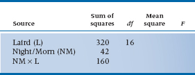
3. For the following designs and ANOVA tables, you get to fill in the blanks:

a. Seventeen Scottish lairds are assembled in the manor, plied with a “wee dram o’ the malt” all night long, then asked to rate their state of euphoria (1) the night before and (2) the morning after.

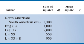
b. An entomologist (bug freak) counts the number of spikes on the legs of North American and South American horned cockroaches (Stylopyga orientalis, yet another Japanese import!) to see if they have different lineages. The bug freak has 20 bugs per group, and 6 legs per bug.

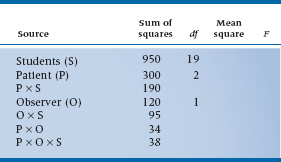
c. Twenty medical students are observed and rated on five different patient workups. Each work-up is observed by two staff clinicians.

How to Get the Computer to Do the Work for You

Because repeated-measures ANOVAs are some what more complex than straight factorial ANOVAs, we’re going to break with tradition a bit and show the actual contents of the computer commands for the analyses we did in this chapter. We’ll use the most complicated analysis, in which there are two groups (Administrative/Research); three drugs; and two types of each drug (Brand/Generic). When we entered the data, we added a variable called Group, which had the value 1 for the administrative group subjects and 2 for the research group subjects.

• From Analyze, choose General Linear Model → Repeated Measures…
  
• Enter Drug <Tab> in the Within-Subjects Factor Name
  
• Enter 3 <Tab> in the Number of Levels box and press
  
• Enter Brndgnrc <Tab> in the Within-Subjects Factor Name
  
• Enter 2 <Tab> in the Number of Levels box and press
  
• Click the button
  
• Click Entrophen, ASA, Tylenol, Acetaminophen, and so on to replace the lines __?__(1,1), __?__(1,2), until the six lines in Within-Subject Variables are filled
  
• Move Group to the Between-Subjects Factor(s) box
  
• Click

The results are spread out in a number of places. Any repeated-measures effect, any interactions with those effects, and the associated error term are within a box labeled Tests of Within-Subjects Contrasts. Any between-subjects effects, interactions not involving within-subject effects, and the error term are in a separate box called Tests of Between-Subjects Effects. This error term corresponds to the Subject effect in Table 11–3.

¹ Actually, hemorrhoids aren’t all bad. After all, it takes two things to be a consultant—them and grey hair. The grey hair makes you look distinguished and the hemorrhoids make you look concerned.

² Literally inflammation of the muscles of the gluteus maximus. Not to be confused with myalgic encephalitis, which was the Latin name briefly adopted for Chronic Fatigue Syndrome. As near as we can tell, it has something to do with having a muscle in the head.

³ I never was much good at arithmetic even back in grade school. “Mr. Norman, count to 10.” “OK, teacher. One, uh, two, uh, multiple.”

⁴ Note from long-suffering coauthor: “It’s about bloody time!”

⁵ Note that, to use the terminology we came across in Chapter 9, since both brand name and generic drugs have comparable formulations, we can claim that Brand/Generic is crossed with the drug. We’ll deal with this later.

⁶ To ensure that committee type is a true between-subjects factor, we must ensure that there are different folks in each group. We could, of course, try to find a situation in which the same people are on both an administrative and a research committee, but then it would be another within-subject factor.

⁷ It’s not essential to have the same number of people in each committee type; we did it just for convenience.

⁸ This presents an ideal situation to cook the data as we see fit. We will.

⁹ After all we’ve put you through in this chapter, the answer may well be “Not.”

¹⁰ We do, however, restrict this to repeated measurements of the same quantity—weight, serum sulphur, or whatever—usually at different points in time. Many studies do make repeated observations on subjects, but of different variables, such as grip strength, morning stiffness, joint count, sedimentation rate, and so on, for arthritic patients. For this situation, use multivariate statistics, covered in later chapters.

¹¹ Note that if a baseline measurement were made, this should not be treated as another level of the time factor. More appropriately, this should be used as a covariate and the analysis should be a repeated-measures analysis of covariance (see Chapter 16).

¹² Usually, that is, in psychology and education. Many clinicians, however, seem to think that this approach is a bit of esoterica foisted on them recently by zealous psychometricians. Ironically, nothing could be further from the truth. We found an entire chapter devoted to the intraclass correlation in Fisher’s 1925 statistics book.

¹³ One exception is a Time factor that consists of very different intervals (e.g., Day 1, Day 2, Day 10, Day 30). Then, the assumption of homoscedasticity may break down and, as we’ll see in Chapter 12, it may be better to analyze the data using MANOVA.

Stay updated, free articles. Join our Telegram channel

Join