FIGURE 12-1 Men’s (left side) and women’s (right side) satisfaction scores, depending on who’s on top.

The second problem is that of multiple testing. As we saw in Chapter 5, the probability of finding at least one outcome significant by chance increases according to the formula:

where N is the number of tests we do. If we have two outcome variables (and, hence, have performed two tests), the probability that at least one will be significant by chance at a .05 level is:

If we have five outcomes, the probability is over 22%; by the time we have 10 outcome variables, it would be slightly over 40%. We could try to control this inflation of the alpha level with a Bonferroni correction or some other technique, but, as we discussed in Chapter 8, these tend to be overly conservative. Also, neither the estimate of how many tests would be sig-nificant by chance, nor the corrections for this would take into account the correlations among the dependent variables, which often can be considerable.

A third problem is the converse of the second: rather than finding significance where there is none, we may overlook significant relationships that are present. First, we’ll show that this can happen and then why it can happen. Let’s start off in the usual way, by plotting the data to help us see what’s going on; the results of the males’ satisfaction questionnaires are shown on the left side of Figure 12–1, and those of the females’ satisfaction on the right side of the figure. Using that most sensitive of tests, the calibrated eyeball, it doesn’t look as if much of anything is happening (insofar as the data are concerned, at least)⁵; the distributions of the two groups (positions) seem to overlap quite a bit for both variables.

TABLE 12–1 Results of t-tests between the groups for both variables

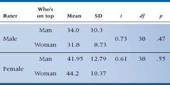
The next step is to do a couple of t-tests on the data, and these are reported in Table 12–1. Again, the groups look to be fairly similar on the two variables; the means are relatively close together, differing by less than half a standard deviation, and only someone truly desperate for a publication would look twice at the significance levels of the t-tests. We could even go so far as to correlate each variable with the grouping variable, using the point-biserial correlation.⁶ This doesn’t help us much either; the correlation between the men’s ratings and position is −0.12, and that for the women’s is an equally unimpressive 0.10.

Now, though, we’ll pull another statistical test out of our bag of tricks and analyze both dependent variables at the same time using a multivariate analysis of variance (MANOVA). We won’t show you the results right now, but trust us that there is now a statistically significant difference between the groups.⁷ So, what’s going on? Why did we find significant results using a multivariate test when it didn’t look as if there was anything happening when we used a whole series of univariate tests? The reason is that the pattern of the variables is different in the two groups. If you go back to Table 12–1, you can see that when men do the rating, they score higher for the male superior position than for the female superior position; but when women do the rating, the situation is reversed—both physically and psychometrically. This couldn’t be seen when we looked at each variable separately. It’s analogous to the advantage of a factorial design over separate one-way ANOVAs: with the former, we can examine interactions among the independent variables that wouldn’t be apparent with individual tests; with MANOVA, we can look at interactions among the dependent variables in a way that is impossible with univariate tests.

So, the conclusions are clear: when you have more than one dependent variable, you’re often ahead of the game if you use multivariate procedures. At the end of this chapter, we’ll discuss some limitations to this approach, but for now let’s accept the fact that multivariate statistics are the best way of analyzing multivariate data.

WHAT DO WE MEAN BY “MULTIVARIATE”

We’ve used the term multivariate a few times, and we’ve even defined it—more than one dependent variable—but let’s be more explicit (and confusing). If we went to the bother of checking in a dictionary, we would find that multivariate simply means “many variables.” In Chapter 9, we looked at the interaction among condom brand and circumcision status on estimations of prowess. To most people, this may seem to be multivariate; after all, we’re examining a total of three variables at once. However, statisticians aren’t like most people. They have their own terms that bear only a passing resemblance to English (e.g., “heteroscedasticity” or “polychotomous”), or they use English words in their own unique and idiosyncratic way that the British would likely describe as “quaint.” We already saw that there is nothing inherently normal about the “normal distribution,” and that “regression analysis” doesn’t involving sucking your thumb or recalling a previous incarnation as a Druid princess. In the same way, statisticians have their own meaning for the word “multivariate.” It refers, as we’ve said, to the analysis of two or more dependent variables (DVs) at the same time. In the example we just used, the type of prophylactic and whether or not the person was circumcised are independent variables (IVs), and there was only one DV, prowess. So, to a statistician, this would be a case of univariate statistics—factorial ANOVA—with two IVs and one DV. It would become a multivariate problem if, in addition to looking at prowess, we also measured the duration of the encounter.⁸

What about repeated-measures ANOVA that we slugged through in the last chapter? That’s multiple dependent variables, isn’t it? Well, not actually. It’s multiple observations of the same dependent variable—repeated measures, that is. As it turns out, the mathematics make it a special case of MANOVA, but it’s considered a univariate procedure because it fits the “single dependent variable” rule.

Doesn’t this sound simple and straightforward? That’s a sure sign that something will go awry. The fly in the ointment is that statisticians aren’t consistent. Some of them would call multiple regression a multivariate technique, even though there is only one DV, and it is mathematically identical to ANOVA. Others prefer the term multivariable but, even here, some use the term to refer to many IVs and some just to indicate that many variables—dependent and independent—are involved. For most of us, however, multivariate means more than one DV, and that’s the usage that we’ll adopt.

t FOR TWO (AND MORE)

If we had only one dependent variable, the statistic we would use for this study would be the t-test, which starts with the null hypothesis:

that is, that the means of the two groups are equal. However, we have two dependent variables in the current example, so that each group has two means. In this case, then, the null hypothesis is:

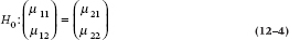
where the first subscript after the μ indicates group membership (1 = Man on Top, 2 = Woman on Top), and the second shows the dependent variable (1 = Male Rater, 2 = Female Rater). What this indicates is that the list of means for Group 1 (the technical term for a list of variables like this is a vector) is equal to the vector of means for Group 2.⁹ In other words, we are testing two null hypotheses simultaneously:

If our study involved a factorial design, such as looking at the effect of being at home versus on a romantic holiday, then we would have another null hypothesis for this new main effect of Setting, and a null hypothesis involving the interaction term of Position by Setting. This is just the same as what we do in the univariate case, except that we are dealing with two or more dependent variables.

When we plot the data for a t-test, we would have two distributions (hopefully normal curves) on the X-axis. The picture is similar but a bit more complicated with multivariate tests. For two variables, we would get an ellipse of points for each group, as in Figure 12–2. If we had three dependent variables, the swarm of points would look like a football (without the laces); four variables would produce a four-dimensional ellipsoid, and so on. These can be (relatively) easily described mathematically, but are somewhat difficult to draw until someone invents three-, four-, or five-dimensional graph paper.

Sticking with the analogy of the t-test, we compare the groups by examining how far apart the centers of the distributions are, where each center is represented by a single point, the group mean. In the multivariate case, we again compare the distance between the centers, but now the center of each ellipse is called the centroid.¹⁰ It can be thought of as the overall mean of the group for each variable; in this case, in two-dimensional space (Male’s rating and Female’s rating). If we had a third variable, we would have to think in three dimensions, and each centroid would consist of a vector of three numbers—the means of the three variables for that group. The logic of the statistical analysis is the same, however: the greater the distance, the more significant the results (all other things being equal).

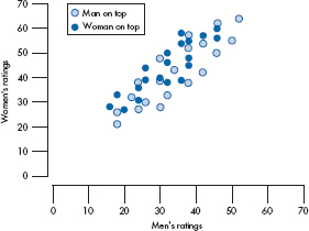
FIGURE 12-2 Scatterplot of the two DVs for both groups.

LOOKING AT VARIANCE

Comparing the means in a t-test is necessary, but not sufficient; we also have to compare the differences between the means to the variances within the groups. Not surprisingly, the same applies in the multivariate case. However, there’s an added level of complexity; in addition to the variances of each of the variables, we also have the covariances between the variables.¹¹ What this means is that instead of having just one number for the variance, we now have a matrix of variance and covariance terms. Not surprisingly, it’s referred to as the variance-covariance matrix (VCV) and looks like:

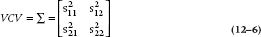
First, note that we just stuck in a third term from matrix algebra, “matrix” itself, which is simply a rectangular array of numbers.¹² Second, the abbreviation for a variance-covariance matrix is either VCV or the symbol ∑. That’s right, it’s the same symbol we use to indicate summation. You’d think that with so many Greek letters lying around that aren’t being used in statistics, statisticians would have thought to use something different, but they didn’t. Usually, the context makes the meaning clear; in addition, the symbol for a matrix is usually printed in boldface, to avoid confusion.¹³

In the VCV matrix, the terms along the main diagonal (s²₁₁ and s²₂₂, where the subscripts are the same) are the variances, and those off the diagonal (s²₁₂ and s²₂₁, where the subscripts are different) are the covariances. Just as with a correlation matrix, the VCV is symmetrical, so the value of s²₁₂ is the same as that for s²₂₁. Needless to say (but we’ll say it anyway), there would be more terms in the VCV matrix if we had more dependent variables: for three variables, we would have three variances and three unique covariances; for four variables, four variances and six covariances, and so on.

Testing for equivalence of the VCV matrices means that the variance of X₁ is the same across all groups; the covariance between X₁ and X₂ is the same; and so forth for all of the variances and all of the covariances. The usual test for homogeneity of the VCV matrices is Box’s M statistic. After some statistical hand waving over the matrices, the number is transformed into either an F-ratio or a χ². If p > .05, then it’s safe to proceed, because the matrices do not differ significantly from each other. However, like many other tests for homogeneity, M is unduly sensitive to differences, especially when the sample size is large. The consequence is that a significant M statistic doesn’t always mean that you have to either stop with the analysis or transform the data; unfortunately, there is nothing but our “feel” for the data to tell us whether the deviation from homogeneity is worth worrying about. Tabachnick and Fidell (2001) offer the following guidelines:

• If the sample sizes are equal, don’t worry about M, because the significance tests are robust enough to handle any deviations from homogeneity
  
• If sample sizes are not equal, and the p associated with M is greater than .001, it’s fairly safe to proceed
  
• If the cell sizes are unequal, and p is less than .001, interpret the results of the MANOVA very cautiously

The consequence of violating the assumption of homogeneity of the VCV matrices if the sample sizes are equal is a slight reduction in the power of the MANOVA. If the sample sizes vary considerably, then a significant M can indicate that the Type I error rate may be either inflated or deflated. Because this depends on which matrices are the most different, it is almost impossible to just look at the data and figure out which it will be.

FROM ANOVA TO MANOVA

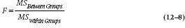
The logic of MANOVA is very similar to that of ANOVA. With the one-way ANOVA, we partition the total variance (the Sum of Squares Total, or SS_Total) into that due to differences between the groups (SS_Between) and the error variance, which is the Sum of Squares within the groups (SS_Within or SS_Error). Then, the F-test looks at the ratio of the explained variance (that due to the grouping factor) to the error (or unexplained) variance, after adjusting for the number of subjects and groups (the Mean Squares). With more complicated designs, such as factorial or repeated-measures ANOVAs, we “simply” split the SS_Total into more sources of variance, such as that due to each factor separately, that due to the interaction between the factors, and that due to measurements over time; divide by the appropriate error term; and get more F-ratios.

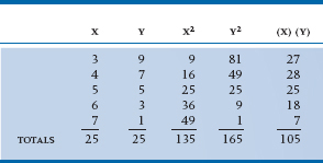
We do exactly the same thing in MANOVA, except that we have more terms to worry about—the relationships between or among the DVs. This is equivalent to expanding the measurement of variance into a variance-covariance matrix when we looked at the assumption of homogeneity of variance. Similarly, we expand the Sum of Squares terms into a corresponding series of Sum of Squares and Cross-Products (SSCP) matrices: SSCP_Total, SSCP_Between, and SSCP_Within. That sounds somewhat formidable, but but it’s something we do all the time in statistics, as we’ll see when we describe the Pearson correlation. A small data set, consisting of two variables (X and Y) and five subjects, is shown in Table 12–2. For each variable, the sum of squares is simply the sum of each value squared.¹⁴ The cross-product is the first value of X multiplied by the first value of Y; these are then added up to form the sum of cross-products. The SSCP matrix for these numbers is therefore:

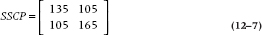
where the off-diagonal cells are the same, since X · Y is the same as Y · X.

The F-test is now just the ratio of the SSCP_Between to the SSCP_Within, after the usual corrections for sample size, number of groups, and the number of DVs. As we’ll see, however, we will run into the ubiquitous problem of multivariate statistics—a couple of other ways to look at the ratios. So, stay tuned.

FINALLY DOING IT

Sad to say, “it” in this case means only running the test (now that we’ve gotten the foreplay out of the way). The first question is, what test do we run? So far, we’ve been referring to the test as MANOVA, and, in fact, that’s how we’ll continue to refer to the test. If you look at older books, however, you’ll see this test is also called Hotelling’s T². Just as a t-test is an ANOVA for two groups (or, in the case of the paired t-test, two related variables), T² is a MANOVA for two groups or two variables. In the years B.C.,¹⁵ it made sense to have a separate test for the two-group case, since there were some shortcuts that could simplify the calculations, which were all done by hand. Now that computers do all the work for us, the distinction isn’t as important, and references to Hotelling’s T² are increasingly rare, and nonexistent in the menus for some computer programs.

If we (finally) run a MANOVA on the satisfaction data, we would get an output similar to that shown in Table 12–3. As we mentioned, the multivariate equivalent of the test for homogeneity of variance is Box’s M, which tests for equivalence of the variance-covariance matrices; this is the first thing we see in the output. The p level shows that the test is not significant, so we don’t have any worries in this regard.

TABLE 12–2 Calculating sums of squares and cross-products

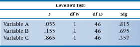
The next set of homogeneity tests belong to Levene,¹⁶ they are univariate tests that look at each of the DVs separately. The usual rule of thumb is that if they are not significant, we can use the results from the MANOVA; if they are significant, then we should stick with univariate tests. In our case, there are no significant differences in the error variances between groups, so it’s safe to use the output labeled Multivariate Tests.

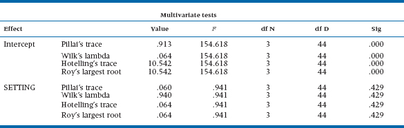
To make our job easier, we can skip the first four lines of the table, those dealing with the intercept. They simply tell us that something is going on, and that the data as a whole deviate from zero.¹⁷ Finally, we arrive where we want to be—a multivariate test of the difference between the groups based on all of the DVs at once. But, as is all too common with multivariate statistics, we don’t have just one test but, rather, four of them! Actually, things aren’t quite as bad as they seem, especially when we have only two groups. As you can see, Hotelling’s trace¹⁸ and Roy’s largest root have the same value; Pillai’s trace¹⁹ and Wilks’ lambda²⁰ add up to 1.0; and with appropriate transformations, all of the tests end up with the same value of F. These relationships don’t necessarily hold true when there are three or more groups, but let’s start off easy.

Because many multivariate tests use Wilks’ Lambda (λ), that’s where we’ll start. As you no doubt remember, the F-ratio for the between-groups effect in an ANOVA is simply:

Analogously, λ is:

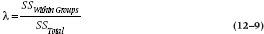
Notice that, for some reason no one except Wilks understands, λ is built upside down; the smaller the within-groups sum of squares (that is, the error), the smaller the value of λ. So, unlike almost every other statistical test we’ll ever encounter, smaller values are better (more significant) than larger ones. What λ shows is the amount of variance not explained by the differences between the groups. In this case, about 6.4% of the variance is unexplained, which means that 93.6% is explained.²¹ Not coincidently, .936 is also the value of Pillai’s trace. In the two-group case, it’s simply (1 − λ), or the amount of variance that is explained.²² Because most people use either Wilks’ λ or Pillai’s criterion, we won’t bother with the other two. When there are more than two groups, Pillai’s trace does not equal (1 − λ), so you’ll have to choose one of them on which to base your decision for significance (assuming they give different results). If you’ve done just a superb job in designing your study, ending up with equal and large sample sizes in each cell, and managed to keep the variances and covariances equivalent across the groups, then use Wilks’ λ. However, if you’re as human and fallible as we are, use Pillai’s criterion, because it is more robust to violations of these assumptions (Olson, 1976), although slightly less powerful than the other tests (Stevens, 1979). In actual fact, however, the differences among all of the test statistics are minor except when your data are really bizarre.

TABLE 12–3 Output from a MANOVA program

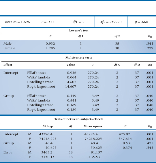
The last part of Table 12–3 gives the univariate tests. Just a little bit of work with a calculator shows that they’re exactly the same as the univariate tests in Table 12–1; square the values of t and you’ll end up with the Fs. These tests are used in two ways. If the assumptions of homogeneity of variance and covariance aren’t met, we would rely on these, rather than on the multivariate tests, to tell us if anything is significant. If we can use the results of the multivariate analysis, these tests tell us which variables are significantly different, in a univariate sense. Hence, they’re analogous to post-hoc tests used following a significant ANOVA. These results are somewhat unusual, in that the multivariate tests are significant but the univariate ones aren’t, indicating that we have to compare the patterns of variables between the groups.

MORE THAN TWO GROUPS

If we had a third group,²³ the output would look very much the same as in Table 12–3. Naturally, the Sums of Squares and Mean Squares would be different, and perhaps the significance levels would also be different (depending on how much or little the participants enjoyed themselves), but the general format would be the same. The major difference in terms of inter-pretation is the Group effect; there will now be two degrees of freedom, reflecting the fact that there are three groups. If the Group effect is significant, then we have the same problem as with a run-of-the-mill, univariate ANOVA: figuring out which groups are significantly different from the others. Fortunately, the method is the same—post-hoc tests, such as Tukey’s HSD. Most programs will do this for you, as long as you remember to choose this option.

DOING IT AGAIN: REPEATED-MEASURES MANOVA

What would be the MANOVA equivalent of a repeated-measures ANOVA? At first glance, it would seem to be two or more dependent variables, both of which are measured on two or more occasions and, in fact, this is one possible design (called a doubly repeated MANOVA). However, even if we have only one DV measured two or three times, it is often better to use a repeated-measures MANOVA than an ANOVA. There are two reasons for this. The first is that, although between-subjects designs are relatively robust with respect to heterogeneity of variance across groups, within-subjects designs are not, resulting in a higher probability of a Type I error than the α level would suggest (LaTour and Miniard, 1983). The second reason is that with ANOVA, there is an assumption of sphericity—that for each DV, the variances are equal across time, as are the correlations (that is, the correlation between the measures at Time 1 and Time 2 is the same as between Time 2 and Time 3 and is the same as between Time 1 and Time 3). Most data don’t meet the criterion of sphericity, and this is especially true when the time points aren’t equally spaced (such as measuring a person’s serum rhubarb level immediately on discharge, then one week, two weeks, four weeks, and finally six months later). It’s more likely that there’s a higher correlation between the measures at Week 1 and Week 2 than between Week 1 and Month 6. Repeated-measures MANOVA, however, treats each time point as if it were a different variable, so the assumption of sphericity isn’t required.

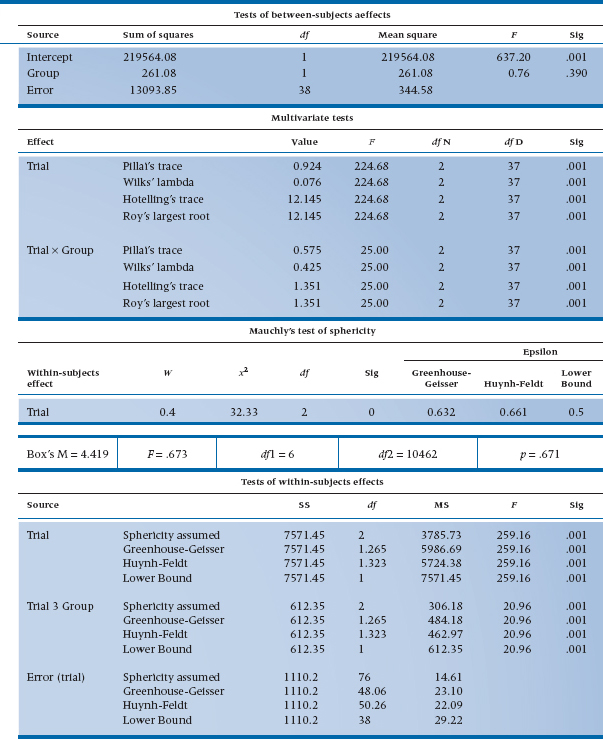
To keep things a bit simpler, we’ll go back to using two groups, and modify our study a bit by having only one rater,²⁴ but we’ll repeat the experiment three times, so we have three time points. The design, then, is a 2 (Who’s on Top) by 3 (Trials) factorial. The results are shown graphically on Figure 12–3, and the computer output appears in Table 12–4.

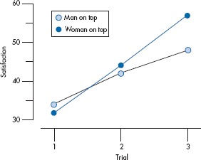
FIGURE 12-3 Repeated measures of satisfaction for the two groups.

The first part of the table gives the results for the between-subjects effect, which in this case is Group or Position. This is actually a univariate test, a one-way ANOVA, in which all of the trials are averaged. In this case, the F is not significant, showing that, overall, position doesn’t make a difference.²⁵

Next, we see the multivariate tests for the within-subjects factors and the interactions between the within-subjects and the between-subjects factors. In this example, we have only one within-subject factor (Trials) and one interaction term (Trials by Group). The same comments apply to this output as previously with regard to the meaning of the four different tests: they all yield the same F-test when there are two groups, and stick with Pillai’s trace or Wilks’ lambda. In this example, there is an overall Trials effect and a significant interaction. If we go back to Figure 12–3, it appears that when summing over Groups, the ratings increase over time; and women’s ratings start somewhat lower but increase more than men’s.²⁶

Following this, we have univariate tests for the within-subject factor, used if Box’s M shows us we should be concerned about the assumption of equality of the covariance matrices. The same general guidelines apply that we discussed before: don’t worry about this if the sample sizes are equal or p > .001. If we do feel that it’s more appropriate to use the univariate tests, then we first have to look at the test of sphericity, known as Mauchly’s W. For the purposes of significance testing, W is transformed into an approximate χ² test. If it is not significant (and you have a sufficient sample size), then we can proceed with abandon, using the appropriate lines in the succeeding tables. If it is significant (as it is here), then the numerator and denominator degrees of freedom for the F-tests are “adjusted” by some value, which is referred to as ε (epsilon). As is so often the case, we have more adjustments than we can use. The most conservative one is the Lower Bound, which assumes the most extreme departure from sphericity.²⁷ The Huynh-Feldt adjustment is the least conservative, with the Greenhouse-Geisser adjustment falling in between. Most people use the Greenhouse-Geisser value, except when the sample size is small, in which case the Huynh-Feldt value is used.²⁸

TABLE 12–4 Output from a repeated-measures MANOVA program

The caveat we added in the previous paragraph about W (“and you have a sufficient sample size”) is one that holds true for every statistical test trying to prove a null hypothesis: the result may not be significant if the sample size is small, and there just isn’t the power to reject the null of sphericity. The trouble is, nobody knows how much is enough,²⁹ so if your sample size is on the low side, you’d be safer to use one of the correction factors.

ROBUSTNESS

We mentioned earlier, when discussing tests of homogeneity of the VCV matrices, that MANOVA is relatively robust to violations here, especially if the group sizes are equal. With that same proviso of equal sample size, it is also relatively robust to deviations from multivariate normality. “Relatively” means two things: if the degrees of freedom associated with the univariate error terms are over 20, and if the deviation from normality is due to skewness, you can get away with almost anything. However, if the df_Error is less than 20, or if the nonnormality is due to outliers, then it would be safer to trust the results of the univariate tests, trim the data to get rid of the outliers,³⁰ or use ranks instead of the raw data (discussed below). It’s also a reminder (as if one were necessary) to plot your data before you do anything else to make sure you don’t have outliers or any other pathologic conditions.

Is there anything we can’t get away with if we have large and equal groups? There are two things we can’t mess around with—random sampling and independence of the observations. As with most statistical techniques, MANOVA assumes that the data come from a random sample of the underlying population, and that the scores for one person are independent of those for all other people. If you violate either of these, the computer will still blithely crunch the numbers and give you an answer, but the results will bear little relationship to what’s really going on.

POWER AND SAMPLE SIZE

As we have seen, the first test that’s performed when we do a MANOVA is a test for homogeneity of the VCV matrices. For this test to run, we must have more subjects than variables in every cell (Tabachnick and Fidell, 1996). But, this is an absolute minimum requirement. There are tables for estimating sample size, based on the number of groups, variables, and power (Läuter, 1978), and some of them appear in Appendix N. These tables first appeared in a very obscure journal from what was once East Germany, so we’re not sure if they are legitimate or part of a conspiracy to undermine capitalist society by having the West’s researchers waste their time with under-or overpowered studies. In any case, we offer them for your use.³¹ Going the other way, Appendix O (adapted from Stevens, 1980) gives the power for the two-group MANOVA (Hotelling’s T²) for different numbers of variables, sample sizes, and effect sizes.

For the most part, MANOVAs are less powerful than univariate tests. This can result in the anomalous situation that some or all of the univariate tests come out significant, but multivariate tests such as Pillai’s trace are not significant.³²

There is one issue that has bedeviled statisticians (and us, too) ever since MANOVA was developed: if the overall F-test is significant, is it necessary to adjust the α level for the post-hoc analyses that examine which specific variables differ between or among the groups? The answer, as has been the case so often in this book, is a definitive, “Yes, no, and maybe.” Some people have vehemently argued that a significant omnibus test “protects” the α levels of the post-hoc tests, so that no adjustment is necessary. There are just as many people on the other side, saying that multiple testing is multiple testing, so a Bonferroni-type adjustment is required.

The problem is that both sides are right, but under different conditions. If the null hypothesis is true for all of the DVs (a situation called the complete null hypothesis), then α is indeed protected, and there’s no need to adjust for the fact that you are doing a number of ANOVAs on the individual variables after the fact.³³ However, if the null hypothesis is true for some of the variables but not for others (the partial null hypothesis), then α is not protected, and an adjustment for multiplicity is required. The problem is that you never know which is the case, even based on the results of the univariate F-tests (Jaccard and Guilamo-Ramos, 2002). So, it’s safest to assume that you’re dealing with the partial null hypothesis, and make the adjustment.

WHEN THINGS GO WRONG: DEALING WITH OUTLIERS

As we’ve mentioned, MANOVA can’t handle data with outliers very well. If you’re reluctant to trim the data and still want to use a multivariate procedure, an alternative exists for the one-way test. First, transform your raw data into ranks; if there are n₁ subjects in Group 1 and n₂ subjects in Group 2, then the ranks will range from 1 to (n₁ + n₂) for each variable. Then, run MANOVA on the rank scores. Finally, multiply the Pillai trace (V) by (N − 1), and check the results in a table of χ², with df = p (k − 1), where p is the number of variables and k the number of groups (Zwick, 1985).

EFFECT SIZE

There are actually at least two effect sizes; one for the MANOVA as a whole, and then one for the individual main effects. As we mentioned, Wilks’ λ is a measure of how much variance is not accounted for, so ES is 1 − λ, or Pillai’s trace. For the main effects and interactions, use η² or ω², as we described in Chapter 8.

A CAUTIONARY NOTE

From all of the above, it may sound as if we should use MANOVA every time we have many dependent measures, and the more the better. Actually, reality dictates just the opposite. The assumption of homogeneity of the VCV matrices is much harder to meet than the assumption of homogeneity of variance; so, it’s more likely that we’re violating something when we do a MANOVA. Second, the results are often harder to interpret, because there are more things going on at the same time. Third, as we’ve seen, we may have less power with multivariate tests than with univariate ones. The best advice with regard to using MANOVA is offered by Tabachnick and Fidell (1983), who are usually strong advocates of multivariate procedures. They write:

Because of the increase in complexity and ambiguity of results with MANOVA, one of the best overall recommendations is: Avoid it if you can. Ask yourself why you are including correlated DVs in the same analysis. Might there be some way of combining them or deleting some of them so that ANOVA can be performed? (p. 230)³⁴

If the answer to their question is “No,” then MANOVA is the way to go—but, don’t throw everything into the pot. The outcome variables included in any one MANOVA should be related to each other on a conceptual level, and it’s usually a mistake to have more than six or seven at the most in any one analysis.

REPORTING GUIDELINES

For a between-subjects design, you can report the results pretty much as if it were a run-of-the-mill ANOVA. It’s not really necessary to report the statistics regarding the intercept, because in most cases, it doesn’t mean much. However, you should also report Wilks’ γ and its transformed value of F (with, of course, the proper df). Within the text, you should report whether or not the tests for homogeneity of the variance–covariance matrix and normality were significant.

For repeated measures designs, life is a bit more complicated. In addition to what we said above, you also have to report Mauchly’s W (best to report the χ² equivalent, with its df). If it’s not significant, then that’s it. But, if it is significant, you must also state which adjustment you used (lower bound, Greenhouse-Geisser, or Huynh-Feldt) and its value.

WRAPPING UP

Taking Tabachnick and Fidell’s advice to heart, we should try to design studies so that MANOVA isn’t needed: we should rely on one outcome variable, or try to combine the outcome variables into a global measure. If this isn’t possible, then MANOVA is the test to use. Analyzing all of the outcomes at once avoids many of the interpretive and statistical problems that would result from performing a number of separate t-tests or ANOVAs. We pay a penalty in terms of reduced power and more complicated results, but these are easier to overcome than those resulting from ignoring the correlations among the dependent variables.

EXERCISES

1. For the following designs, indicate whether a univariate or a multivariate ANOVA should be used.

a. Scores on a quality-of-life scale are compared for three groups of patients: those with rheumatoid arthritis, osteoarthritis, and chronic fatigue syndrome.

b. Each of these patient groups is divided into males and females as another factor.

c. All of these groups are tested every 2 months for a year.

d. The same design as 1.a, but now the eight subscales of the quality-of-life scale are analyzed separately.

e. Same design as 1.b, but using the eight subscales.

f. Same as 1.c, but with the subscales.

2. If the three groups did not differ with regard to their quality of life, and if the eight subscales were analyzed separately, what is the probability that at least one comparison will be significant at the .05 level by chance?

3. Based on the results of Box’s M, you should:

a. proceed with the analysis without any concern.

b. proceed, but be somewhat concerned.

c. stop right now.

4. Based on the results of Levene’s test, you should:

a. use the results of the multivariate tests.

b. use the results of the univariate tests.

5. Looking at the output from the multivariate tests:

a. Is there anything going on?

a. Does the variable SETTING have an effect?

How to Get the Computer to Do the Work for You

• From Analyze, choose General Linear Model →Multivariate…
  
• Click the variables you want from the list on the left, and click the arrow to move them into the box labeled Dependent Variables
  
• Choose the grouping factor(s) from the list on the left, and click the arrow to move them into the box labeled Fixed Factor(s)
  
• If you have more than two groups, click the button and select the ones you want [good choices would be LSD, Tukey, and Tukey’s-b], and then click the button
  
• Click the button and check the statistics you want displayed. The least you want is Homogeneity Tests; if you haven’t analyzed the data previously, you will also want Descriptive Statistics and perhaps Estimates of Effect Size
  
• If you have a repeated-measures design, use the instructions at the end of Chapter 11.

¹ If you’re not sure how this question relates to the test, check the Glossary under “MANOVA.”

² We will not use the term “in the superior position,” because that will only cause havoc among those who want to generalize the term to other situations.

³ We recognize that restricting this study to situations involving only two partners may impose limitations for some people, but it is necessary to keep the analysis simple.

⁴ Don’t be scared off. We don’t understand it too well, either, so we’ll avoid it as much as we can. You’ll have to know some of the language, but since this is your first time, we’ll be gentle.

⁵ Looking at the magnitudes of those evaluations, it doesn’t look as if much is happening elsewhere, either.

⁶ Which, as you no doubt remember, is simply a Pearson correlation of one continuous variable (each satisfaction scale) with a dichotomous one (who’s on top?).

⁷ If you don’t trust us, you can skip ahead a few pages to Table 12–3 and check for yourself. Now, aren’t you sorry you doubted us?

⁸ A polite term for “it.”

⁹ You’ve just been introduced to your first term in matrix algebra, “vector.” See, that was painless, wasn’t it? There actually is a link between the use of the term vector in matrix algebra and in disease epidemiology, obscure though it may be: both are represented symbolically by arrows.

¹⁰ That’s your second term in matrix algebra.

¹¹ A covariance is similar to a correlation between two variables, except that the original units of measurement are retained, rather than transforming the variables to standard scores first, as is done with correlations. It reflects the variance shared by the two variables.

¹² We didn’t want to tell you at the time, but now that you’ve progressed this far, you can finally know: you’ve been dealing with matrices throughout the book. Any time you saw a table listing subjects down the side and variables across the top, you were looking at a data matrix.

¹³ Unless, of course, you forget whether it’s sums or matrices that are printed in boldface.

¹⁴ Makes sense, doesn’t it?

¹⁵ That’s Before Computers; non-Christians prefer the term B.C.E., for Before Calculating Engines.

¹⁶ Although he lets us use them.

¹⁷ If this ever does come out as nonsignificant, we should question whether we should be in this research game at all or become neo-postmodern deconstructionists, so that no one will ever know that our hypotheses amount to nothing.

¹⁸ Also called the Hotelling-Lawley trace, or T.

¹⁹ Which is also called the Pillai-Bartlett trace, or V.

²⁰ A.k.a. Wilks’ likelihood ratio, or W. (Ever get the feeling that everything is called something else in this game?)

²¹ If you didn’t suspect it before, this should convince you that these are artificial data; if we did any study that accounted for 94% of the variance, our picture would show us holding Nobel prize medals, not a lousy cardboard maple leaf.

²² Pillai’s trace is also equivalent to η² (eta-squared), which is the usual measure of variance accounted for in ANOVAs.

²³ You can use your imagination for this, as long as it doesn’t involve more than two people; that would require another dependent variable (and perhaps a larger bed). As a hint, a bed isn’t de rigueur.

²⁴ You can determine for yourself whether the scores show it’s a man or a woman doing the ratings.

²⁵ And if you believe that, we have some property in Florida we’d like to sell you.

²⁶ As before, we leave it to you to figure out the meaning of this.

²⁷ It’s called the Lower Bound because it is the lowest value that ε can have: 1 / (k −1), where k is the number of groups. The maximum value of ε is 1.0, indicating homogeneity.

²⁸ If the Lower Bound adjustment is rarely used, then why is it printed out? Probably because the programmer’s brother-in-law devised it.

²⁹ At least in the area of statistics.

³⁰ “Trimming” is how you can get rid of data you don’t want and still get published, as opposed to saying that you simply disregarded those values you didn’t like.

³¹ The authors (hereinafter referred to as the Parties of the First Part) do verily state, declare, and declaim that all warranties, expressed or implied, assumed by users of these Tables (Parties of the Second Part) are hereby and forthwith null and void.

³² Proving yet again (as if further proof were needed) that there ain’t no such thing as a free lunch.

³³ And don’t forget that if the null hypothesis is true for all DVs, you’re dealing with a Type I error to begin with.

³⁴ Somewhat poignantly, they answer their own question in the next edition of their book: “In several years of working with students … we have been royally unsuccessful at talking our students out of MANOVA, despite its disadvantage” (Tabachnick and Fidell, 1996, p. 376).

Stay updated, free articles. Join our Telegram channel

Join