This is just longer than what we had before, not fundamentally different. A reasonable next step would be to graph the data. However, no one has yet come up with six-dimensional graph paper, so we’ll let that one pass for the moment. Nevertheless, we will presume, at least for now, that were we to graph the relationship between ROM and each of the independent variables individually, an approximately straight line would be the final result.

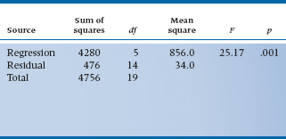
TABLE 14–1 Analysis of variance of prediction of ROM from five independent variables

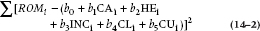
We can then proceed to stuff the whole lot into the computer and press the “multiple regression” button. Note that “the whole lot” consists of a series of 20 data points on this six-dimensional graph paper, one for each of the 20 Yuppies who were in the study. Each datum is in turn described by six values corresponding to ROM and the five independent variables. The computer now determines, just as before, the value of the bs corresponding to the best-fit line, where “best” is defined as the combination of values that result in the minimum sum of squared deviations between fitted and raw data. The quantity that is being minimized is:²

We will call this sum, as before, the Sum of Squares (Residual) or SS_res.

Of course, two other Sums of Squares can be extracted from the data, Sum of Squares (Regression), or SS_reg, and Sum of Squares (Total), or SS_tot.

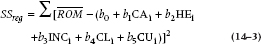
Although this equation looks a lot like SS_res, the fine print, particularly the bar across the top of ROM instead of the i below it, makes all the difference. SS_res is the difference between individual data, ROM_i, and the fitted value; SS_reg is the difference between the fitted data and the overall grand mean Finally, SS_tot is the difference between raw data and the grand mean:

And of course, we can put it all together, just as we did in the simple regression case, making an ANOVA table (Table 14–1).

Several differences are seen between the numbers in this table and the tables resulting from simple regression in the previous chapter. In fact, only the Total Sum of Squares (4756.0) and the df (19) are the same. How can such a little difference make such a big difference? Let’s take things in turn and find out.

1. Sum of Squares—Although the Total Sum of Squares is the same as before, the Sum of Squares resulting from regression has actually gone up a little, from 3892 to 4280. This is actually understandable. In the simple regression case, we simply added up the five subscores to something we called CHICC. Here we are estimating the contribution of each variable separately so that the overall fit more directly reflects the predictive value of each variable. In turn, this improves the overall fit a little, thereby increasing the Sum of Squares (Regression) and reducing the Sum of Squares (Residual) by the same amount.
   
2. Degrees of Freedom—Now the df resulting from regression has gone from 1 to 5. This is also understandable. We have six estimated parameters, rather than two, as before; one goes into the intercept. The overall df is still 19, with 5 df corresponding to the coefficients for each variable. Then, because the overall df must still equal the number of data −1, the df for the residual drops to 14.
   
3. Mean Squares and F-ratio—Finally, the Mean Squares follow from the Sum of Squares and df. Because Sum of Squares (regression) uses 5 df, the corresponding Mean Square has dropped by a factor of nearly four, even though the fit has improved. This then results in a lower F-ratio, now with 5 and 14 df, but it is still wildly significant.

Significant or not, this is one of many illustrations of the Protestant Work Ethic as applied to stats: “You don’t get something for nothing.” The cost of introducing the variables separately was to lose df, which could reduce the fit to a nonsignificant level while actually improving the fitted Sum of Squares. Introducing additional variables in regression, ANOVA, or anywhere else can actually cost power unless they are individually explaining an important amount of variance.

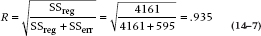
We can now go the last step and calculate a correlation coefficient:

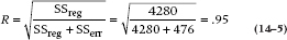
As you might have expected, this has gone up because the Sum of Squares (Regression) is larger. Note the capital R; this is called the Multiple Correlation Coefficient to distinguish it from the simple correlation. But the interpretation is the same.

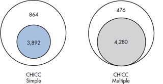
FIGURE 14-1 Proportion of variance (shaded) from simple regression of CHICC score and multiple regression of individual variables. The numbers represent the relevant Sum of Squares.

The Multiple Correlation Coefficient (R) is derived from a multiple regression equation, and its square (R²) indicates the proportion of the variance in the dependent variable explained by all the specified independent variables.

As always, a graphical interpretation displays activities of the sums of squares. In Figure 14–1, we have shown the proportion of the Total Sum of Squares resulting from regression and residual. As we already know, a bit of difference exists, with the multiple regression taking a bit more of the pie.

So that’s it so far. You might rightly ask what the big deal is because we have not done much else than improve the fit a little by estimating the coefficients singly, but at the significant cost of df. However, we have not, as yet, exploited the specific relationships among the variables.

Types of Variables

Before we go much further, let’s discuss the types of variables that we can use in multiple regression. The only requirement is that the dependent variable be normally distributed (to be more precise, that the errors or residuals—which we’ll discuss later—are normally distributed). Other forms of regression, such as logistic regression or Poisson regression (which are discussed in the next chapter), allow for different distributions of the dependent variable. What about the predictor variables? The bad news is that it’s assumed that they’re measured without any error. This is like the Ten Commandments—something we all aspire to but is impossible to achieve in real life (we’ll leave it to you to decide which ones to break). So, as with those injunctions, we’ll acknowledge this one exists and then promptly forget about it. Its only meaningful implication is that regression is a large sample procedure; with small samples, the error has a large effect, but it becomes less important as the sample size increases.

The good news is that there are no assumptions about the distributions of the predictors. Want to use normally distributed variables? Great. You have dichotomous ones? Sure, go right ahead. About the only type we can’t use are nominal variables, where the coding is arbitrary, but we’ll tell you how to handle those later in the chapter. This means that if your predictors aren’t normally distributed, you don’t have to do any fancy transformations to make them normal.

RELATIONSHIPS AMONG INDIVIDUAL VARIABLES

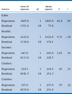
Let’s backtrack some and take the variables one at a time, doing a simple regression, as discussed previously. If you permit a little poetic license, the individual ANOVAs (with the corresponding correlation coefficients) would look like Table 14–2. These data give us much more information about what is actually occurring than we had before. First, note that the total sum of squares is always 4756, as before. But CARS alone is most of the sum of squares and has the correspondingly highest simple correlation. This is as it should be; it was clinical observations about cars that got us into this mess in the first place. HEALTH comes next, but it has a negative simple correlation; presumably if you get enough exercise, your muscles can withstand the tremendous stresses associated with Beemer Knee. INCOME is next, and still significant; presumably you have to be rich to afford cars and everything else that goes with a Yuppie lifestyle. Last, CUISINE and CLOTHES are not significant, so we can drop them from further consideration.

TABLE 14–2 ANOVA of regression of individual variables

Although we confess to having rigged these data so that we wouldn’t have to deal with all the complications down the road, the strategy of looking at simple correlations first and eliminating from consideration insignificant variables is not a bad one. The advantage is that, as we shall see, large numbers of variables demand large samples, so it’s helpful to reduce variables early on. The disadvantage is that you can get fooled by simple correlations—in both directions.

At first blush, you might think that we can put these individual Sums of Squares all together to do a multiple regression. Not so, unfortunately. If we did, the Regression Sum of Squares caused by just the three significant variables would be:

Not only is this larger than the Sum of Squares (Regression) we already calculated, it is also larger than the total Sum of Squares! How can this be?

Not too difficult, really. We must recognize that the three variables are not making an independent contribution to the prediction. The ability to own a Beemer and belong to exclusive tennis clubs are both related to income—the three variables are intercorrelated. This may suggest that income causes everything, but then real income may lead to a Rolls, and legroom is not an issue in the driver’s seat of a Rolls.³ We are not, in any case, concerned about causation, only correlation, and as we have taken pains to point out already, they are not synonymous. From our present perspective, the implication is that, once one variable is in the equation, adding another variable will account only for some portion of the variance that it would take up on its own.

As a possibly clearer example, imagine predicting an infant’s weight from three measurements—head circumference, chest circumference, and length. Because all are measures of baby bigness, chances are that any one is pretty predictive of baby weight. But once any of them is in the regression equation, addition of a second and third measurement is unlikely to improve things that much.

We can also demonstrate this truth graphically. First, consider each variable alone and express the proportion of the variance as a proportion of the total area, as shown in Figure 14–2. Each variable occupies a proportion of the total area roughly proportional to its corresponding Sum of Squares (Regression). Note, however, what happens when we put them all together as in the lower picture. This begins to show quantitatively exactly why the Sum of Squares (Regression) for the combination of the three variables equals something considerably less than the sum of the three individual sums of squares. As you can see, the individual circles overlap considerably, so that if, for example, we introduced CARS into the equation first, incorporating HEALTH and INCOME adds only the small new moon-shaped crescents to the prediction. In Figure 14–3 we have added some numbers to the circles.

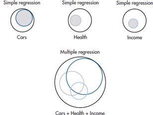
FIGURE 14-2 Proportion of variance from simple regression of Cars, Health, and Income, and multiple regression.

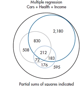
FIGURE 14-3 Proportion of variance from multiple regression with partial sums of squares.

We already know that the Sum of Squares (Regression) for CARS, HEALTH, and INCOME are 3405, 1622, and 643, respectively. But Figure 14–3 shows that the overall Sum of Squares (Regression), as a result of putting in all three variables, is only SS (Total) − SS (Err) = (4756 − 595) = 4161. (Alternatively, this equals the sum of all the individuals areas [2180 + 830 + 212 + 183 + 508 + 72 + 176] = 4161.) For thoroughness, the new multiple correlation, with just these three variables, is:

PARTIAL F-TESTS AND CORRELATIONS

Partial F-Tests

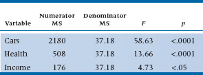
We can now begin identifying the unique contributions of each variable and devising a test of statistical significance for each coefficient. The test of significance is based on the unique contribution of each variable after all other variables are in the equation. So, for the contribution of CARS, the unique variance is 2180; for HEALTH, it’s 508; and for INCOME, it is 176. Now we devise a test for the significance; each contribution called, for fairly obvious reasons, a partial F-test. Its formula is as follows:

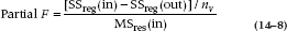
where (in) is with the variables in the equation, (out) is with the variables out of the equation, and n_v is the number of variables.

The partial F-test is the test of the significance of an individual variable’s contribution after all other variables are in the equation.

The numerator of this test is fairly obvious: the Sum of Squares explained by the variables added, divided by the number of variables, or the Mean Square due to variables added.

The denominator of the test is a bit more subtle. What we require is an estimate of the true error variance. As any of the Sums of Squares within the “regression” circles is actually variance that will be accounted for by one or another of the predictor variables, the best guess at the Error Sum of Squares is the SS (Err) after all variables are in the equation, in this case equal to 595. In turn, the Mean Square is then divided by the residual df, now equal to (19 − 3) = 16. So, the denominator for all of the partial F-tests is 595 ÷ 16 = 37.18, and the tests for each variable are in Table 14–3.

Partial and Semipartial Correlations

Another way to determine the unique contribution of a specific variable, after the contributions of the other variables have been taken in account, is to look at the partial and semipartial (or part) correlations. Let’s say we have a dependent variable, z, and two predictor variables, a and b. The partial correlation between a and z is defined as:

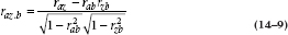
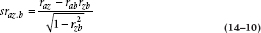
The cryptic subscript, r_az.b, means the correlation between a and z, partialling out the effects of b. This statistic tells us the correlation between a and z, with the contribution of b removed from both of the other variables. However, for our purposes, we want the effect of b removed from a, but we don’t want it removed from the dependent variable. For this, we need what is called the semipartial correlation, which is also known by the alias, the part correlation. Its numerator is exactly the same as for the partial correlation, but the denominator doesn’t have the SD of the partialled scores for the dependent variable:

Partial and semipartial correlations highlight one of the conceptual problems in multiple regression. On the one hand, the more useful variables we stick into the equation (with some rare exceptions), the better the SS_reg, R, and R², all of which is desirable. On the other hand (and there’s always another hand), the more variables in the equation, the smaller the unique contribution of a particular variable (and the smaller its t-test). This is also desirable, because the contribution of any one variable is not usually independent of the contributions of others. We could, in fact, end up with the paradoxical situation that none of the predictors makes a significant unique contribution, but the overall R is “whoppingly” significant. We’ll return to some of these pragmatic issues in a later section.

TABLE 14–3 Partial F tests for each variable

bS AND βS

As you may have noticed, we have been dealing with everything up to now by turning them into sums of squares. The advantage of this strategy is that all the sums of squares add and subtract, so we can draw pretty pictures showing what is going on. One disadvantage is that we have lost some information in the process. We did discuss the basic idea in Chapter 13, where we were dealing with simple regression. In particular, we have not actually talked about the b coefficients, which is where we began. In the last chapter, the significance of each individual b coefficient is tested with a form of the t-test, creating a table like Table 14–4. Further, the t-test is simply the square root of the associated partial F value, which we already determined using Equation 14–8.

The coefficient, b, also has some utility independent of the statistical test. If we go back to the beginning, we can put the prediction equation together by using these estimated coefficients. We might actually use the equation for prediction instead of publication. For our above example, the prediction equation from the CHICC variables could be used as a screening test to estimate the possibility of acquiring Beemer Knee.

The b coefficients can also be interpreted directly as the amount of change in Y resulting from a change of one unit in X. For example, if we did a regression analysis to predict the weight of a baby in kilograms from her height in centimeters, and then found that the b coefficient was .025, it would mean that a change in height of 1 cm results in an average change of weight of .025 kg, or 25 g. Scaling this up a bit, a change of 50 cm results in an increase in weight of 1.25 kg.

Next in the printout comes a column labeled β. “Beta?” you ask. “Since when did we go from samples to populations?” Drat—an exception to the rule. This time, the magnitude of beta bears no resemblance to the corresponding b value, so it is clearly not something to do with samples and populations. Actually, a simple relationship is found between b and β, which looks like this:

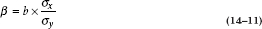
TABLE 14–4 Coefficients and standard errors

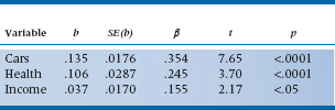
In words, β is standardized by the ratio of the SDs of x and y. As a result, it is called a standardized regression coefficient. The idea is this: although the b coefficients are useful for constructing the regression equation, they are devilishly difficult to interpret relative to each. Going back to our babies, if weight is measured in grams and height in meters, the b coefficient is 10,000 times larger than if weight is measured in kilograms and height in centimeters, even though everything else stayed the same. So by converting all the variables to standard scores (which is what Equation 14–9 does), we can now directly compare the magnitude of the different βs to get some sense of which variables are contributing more or less to the regression equation.

Relative Importance of Variables

Now that we’ve introduced you to bs and βs, the question is which do we use in trying to interpret the relative importance of the variables in predicting the dependent variable (DV)? Let’s briefly recap some of the properties of b and β. We use b with the raw data, and β with standardized data. Because the bs are affected by the scale used to measure the variable (e.g., change cost from dollars to cents and you’ll decrease the b by 100), it’s out of the running. So, at first glance, it may seem as if we should look at the relative magnitudes of the βs to see which predictors are more important. But—and there’s always a “but”—we have to remember one thing: the βs are partial weights. That is, they reflect the contribution of the variable after controlling for the effect of all of the other variables in the equation. Previously, we used the example of predicting an infant’s weight from head circumference, chest circumference, and length. Because the three predictor variables are highly correlated with one another, the unique contribution of each (i.e., its effect after controlling for the other two) would be relatively small. The result is that, for any given variable, its β weight may be quite small and possibly nonsignificant, even though it may be a good predictor in its own right. Indeed, it’s possible that none of the predictors is statistically significant, but the equation as a whole has a high multiple correlation with weight.

Another consequence of the fact that βs are partial weights is that their magnitude is related to two factors: the strength of the relationship between a variable and the dependent variable (this is good), and the mix of other variables in the equation (this isn’t so good). Adding or dropping any of the predictors is going to change the size and possibly the significance level of the weights. This means that we also have to look at the correlations between each independent variable (IV) and the predicted value of the DV (i.e., Ŷ); what are called structure coefficients (r_s). But here again, there may be problems. There are times (thankfully, relatively rare) where the structure correlation is very low, but the β weight is high. This occurs if there is a “suppressor” variable that contaminates the relationships between the other predictor variables and the DV. For example, we may have a test of math skills that requires a student to read the problems (you remember the type: “Imagine that there are two trains, 150 miles apart. Train A is approaching from the east at 100 mph, and Train B is coming from the west traveling at 80 mph. How long will it take before they crash into each other?”).⁴ If some kids are great at math but can’t read the back of a cereal box, then language skills⁵ will suppress the relationship between other predictors and scores on a math exam.

So, which do we look at—the β weights or the r_ss? The answer is “Yes.” If the predictors are uncorrelated with one another, it doesn’t matter; the β and r_ss will have the same rank ordering, and differ only in magnitude. When they are correlated (and they usually are), we have to look at both. If β is very low, but r_s is high, then that variable may be useful in predicting the DV, but its shared predictive power was taken up by another IV. In other words, the variable may be “important” at an explanatory level, in that it is related to the DV, but “unimportant” in a predictive sense because, in combination with the other variables in the equation, it doesn’t add much. On the other hand, if β is high but r_s² is low, then it may be a suppressor variable (Courville and Thompson, 2001).

But, how do we examine the correlation between a variable and Ŷ? One way is to run the regression and save the predicted values, and then get the correlations between them and all of the predictor variables. Another way, that may actually be easier, is to calculate them directly:

where is the correlation between the predictor X_i and the DV, and R is the multiple correlation. This formula also tells us two important things about the r_ss. First, notice that only the IV that we’re interested in is the numerator, not any of the other IVs. That means that structure coefficients are not affected by multi-collinearity. Second, because each r_s is simply the zero-order correlation between the IV and the DV divided by a constant (R), the rank order of the r_ss is the same as that of the r_s. But, because we’re dividing a number less than 1.0, r_s is “inflated” relative to r.

So, why go to the bother to calculate r_ss rather than just use r? In fact, some people (e.g., Pedhazur, 1997) argue that you shouldn’t use them at all because they don’t add any new information. Others argue that r_s is more informative because it tells us the relationship between a predictor variable and the predicted value of Y (i.e., Ŷ), which is really what we’re interested in. Also, structure coefficients play important roles in interpreting other statistics based on the general linear model (which we’ll discuss later), so it’s easier to see the relationship between multiple regression and other techniques.

The bottom line, though, is that whether you use r or r_s to figure out what’s important, the first step is to look at R² and see if it’s worthwhile going any further. If it’s too small to pique your interest, stop right there. Only if it is of sufficient magnitude should you look at the βs and r_ss (or r_s) and decide which variables are important in helping to predict the DV.

GETTING CENTERED

A caveat. This section is not a digression into “new age” psychobabble; there’s enough nonsense written about that already without having us add our two cents’ worth. Rather, it describes a technique that may make the interpretation of the results of multiple regression easier, and help alleviate some of the other problems we may encounter.

If we were to run a regression without thinking about what we’re doing (i.e., the way 99.34% of people do it), we would take our raw data, enter them into the computer, and hit the Run button. When the computer has finished its work, we’ll have a table of bs and βs as we described in an earlier section. Let’s try to interpret these. Remember that the formula we ended up with is:

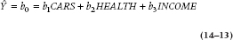
The intercept, b₀, is the value of Beemer Knee we’d expect when all of the IVs have a value of zero. Similarly, b₁ is the effect of Cars on Beemer Knee when the other variables are set equal to zero, and so on for all of the other b coefficients in the equation. Now, we know what it means to have no cars and no income—everyone with kids in university has experienced that. But, what does it mean to have no health? That’s a meaningless concept. It would be even worse if we threw in Age as another predictor; we’d be examining a middle-aged ailment for people who have just been born!

To see how centering can help us interpret the data better, let’s go back to the example of the C¹¹ diet in Chapter 10. Because Captain Casper Casimir’s diet looks so promising, we’ll do a bigger study, comparing 50 men and 50 women, half of whom use the diet and half of whom do not. (Yes, yes, we know that this would normally be analyzed with a 2 × 2 factorial ANOVA, but as we’ll explain in the next chapter, regression and ANOVA are really different ways of doing the same thing.) After months of being or not being on the diet, we weigh these 100 people and get the results shown in Table 14–5. Now, let’s run a multiple regression, where the DV is weight, and the IVs are Gender (1 = Male, 2 = Female) and Group (1 = C¹¹, 2 = Control). The bs that we get are shown in the first line of Table 14–5.

TABLE 14–5 Weights of 50 men and 50 women, half of whom were on the C¹¹ diet

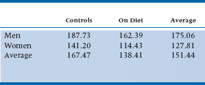
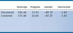
TABLE 14–6 Results of a multiple regression of the C¹¹ study, without (line 1) and with (line 2) centering

Going by what we said before, the intercept is the weight of a person whose gender is 0, and who was in Group 0. Now that really told us a lot, didn’t it? The bs for Program and Gender are equally uninformative, because they are the differences in weight compared with groups that don’t exist. So, we can use the equation to predict the average weight gain or loss for a new individual, but the coefficients don’t tell us much.

Now, let’s use centering, following the recommendations of Kraemer and Blasey (2004). For dichotomous variables, use weights of +½ and −½ instead of 1 and 2, or 0 and 1, or any other coding scheme. So, if we code men as −½ and women as +½; and C¹¹ people as −½ and controls as +½, we’ll get the results shown in the second line of Table 14–6. Suddenly, the numbers become meaningful. The intercept (151.44) is the mean of the whole group, as we see in Table 14–5. The b for Program (26.06) is exactly the difference between the mean weights of the two programs (165.47 for the Controls, and 138.41 for the C¹¹ group); and that for Gender (−47.25) is the difference between the mean weights of men (175.06) and women (127.81).

Centering has other effects, too. With the raw data, there was a significant effect of Gender (p = .023), but neither Program nor the interaction between Program and Gender were significant. Once we center the data, though, Gender becomes even more significant (p < .001), and the effect of Program is significant (p = .0002). As you can see from Table 14–6, centering doesn’t affect the b for the interaction between the variables, nor does it change the significance level. Another advantage, which we won’t elaborate on, is that when multicollinearity (high multiple correlations among the predictor variables, which we’ll discuss in just a bit) is present, centering reduces its ill effects.

So what do we do if the variable is ordinal or interval? Kraemer and Blasey (2004) recommend using the median for ordinal data, and the mean for interval (or ratio) variables. In fact, they argue that, unless there are compelling reasons to the contrary, we should always center the data, which will also help to center our lives.

HIERARCHICAL AND STEPWISE REGRESSION

One additional wrinkle on multiple regression made possible by cheap computation is called stepwise regression. The idea is perfectly sensible—you enter the variables one at a time to see how much you are gaining with each variable. It has an obvious role to play if some or all of the variables are expensive or difficult to get. Thus economy is favored by reducing the number of variables to the point that little additional prediction is gained by bringing in additional variables. Unfortunately, like all good things, it can be easily abused. We’ll get to that later.

Hierarchical Stepwise Regression

To elaborate, let’s return to the CHICC example. We have already discovered that Cuisine and Clothes are not significantly related to ROM, either in combination with the other variables or alone. This latter criterion (significant simple correlation) is a useful starting point for stepwise regression because the more variables the computer has to choose from, the more possibility of chewing up df and creating unreprodicible results.

Physiotherapy research is notoriously under-funded, so our physiotherapist has good reason to see if she can reduce the cost of data acquisition. She reasons as follows:

1. Information on the make of cars owned by a patient can likely be obtained from the Department of Motor Vehicles without much hassle about consent and ethics.⁶
   
2. She might be able to get income data from the Internal Revenue department, but she might have to fake being something legitimate, such as a credit card agency or a charity. This could get messy.
   
3. Data about health, the way she defined it, would be really hard to get without questionnaires or phone surveys.

So if she had her druthers, she would introduce the variables into the equation one at a time, starting with CARS, then INCOME, then HEALTH. This perfectly reasonable strategy of deciding on logical or logistic grounds a priori about the order of entry is called hierarchical stepwise regression. Because it requires some thought on the part of the researcher, it is rarely used.

Hierarchical stepwise regression introduces variables, either singly or in clusters, in an order assigned in advance by the researcher.

What we want to discover in pursuing this course is whether the introduction of an additional variable in the equation is (1) statistically significant, and (2) clinically important. Statistical significance inevitably comes down to some F-test expressing the ratio of the additional variance explained by the new variable to the residual error variance. Clinical importance can be captured in the new multiple correlation coefficient, R², or, more precisely, the change in R² that results from introducing the new variable. This indicates how much additional variance was accounted for by the addition of the new variable.

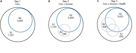
FIGURE 14-4 Proportion of variance from stepwise regression of Cars, Income, and Health. The sums of squares correspond to A, regression from the previous step, B, additional Sum of Squares from pre-sent step, and C, residual Sum of Squares.

All this stuff can be easily extracted from Figure 14–3. We have rearranged things slightly in Figure 14–4. Now we can see what happens every step of the way. In Step 1, we have one independent variable, CARS, and the results are exactly the same as the simple regression of CARS on ROM. The Sum of Squares (Regression) is 3405, with 1 df, and the Sum of Squares (Error) is 1351, with 18 df. The multiple R² is just the proportion of the Sum of Squares explained, 3405 ÷ 4756 = .716 as before, and the F-test of significance is the Mean Square (Regression) ÷Mean Square (Error) = (3405 ÷ 1) ÷ (1351 ÷ 18) = 45.36.

Now we add INCOME. Because all the independent variables are interrelated, this adds only 248 to the Sum of Squares (Regression), for a total of 3653, with 2 df, leaving a Sum of Squares (Error) of 1103 with 17 df. Now the multiple R² is 3653 ÷ 4756 = .768, and the F-test for the addition of this variable is (248 ÷ 1) ÷ (1103 ÷ 17) = 3.822. This is conventionally called the F-to-enter because it is associated with entering the variable in the equation. The alternative is the F-to-remove, which occurs in stepwise regression (discussed later). This score results from the computer’s decision that, at the next step, the best thing it can do is remove a variable that was previously entered.

A subtle but important difference exists between this partial sum of squares and the partial sum of squares for INCOME, which we encountered previously. In ordinary multiple regression, the partials are always with all the other independent variables in the equation, so it equalled only 176. Here, it is the partial with just the preceding variables in previous steps in the equation; consequently, this partial sum of squares is a little larger.

Finally, we throw in HEALTH. This adds 508 to the Sum of Squares (Regression) to bring it to 4161, with 3 df. The Sum of Squares (Error) is further reduced to 595, with 16 df. The multiple R² is now 4161 ÷ 4756 = .875, and the F-test is (508 ÷ 1) ÷ (595 ÷ 16) = 13.66.

All of this is summarized in Table 14–7, where we have also calculated the change in R² resulting from adding each variable. Addition of INCOME accounted for only another 5% of the variance. Although this is not too bad (most researchers would likely be interested in variables that account for 2 to 3% of the variance), this time around it is not significant. How can this be? Recognize that both the numerator and denominator of the F-test are contingent on what has gone before. The numerator carries variance in addition to that already explained by previous variables, and the denominator carries variance that is not explained by all the variables in the equation to this time. When we examined the partial F-tests in Table 14–3, all three variables were in the equation. The additional Sum of Squares resulting from INCOME was 176 instead of 248 because both CARS and HEALTH were in the equation. However, the denominator (the Mean Square [Residual]) was reduced further from 1103 ÷ 17 = 64.9 to 37.18. The net effect was that the partial F-test for introduction of INCOME was just significant in the previous analysis.

This illustrates both the strength and limitations of the stepwise technique. By considering the combination of variables, it is possible to examine the independent effect of each variable and use the method to eliminate variables that are adding little to the overall prediction. Unfortunately, therein also lies a weakness, because the contribution of each variable can be considered only in combination with the particular set of other variables in the analysis.

As we shall see, these problems are amplified when we turn to the next method.

TABLE 14–7 Stepwise regression analysis of ROM against Cars, Income, and Health

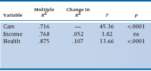
ns = not significant.

Ordinary Stepwise Regression

In this method, the researcher begins by turning over all responsibility for the logical relationship among variables to the machine. Variables are selected by the machine in the order of their power to explain additional variance. The mathematics are the same as used in hierarchical regression described above, except that, at the end of every step, the computer calculates the best next step for all the variables that are not yet in the equation, then selects the next variable to enter based on a statistical criterion. The usual criterion is simply the largest value of the F-to-enter, determined as we did before.

The process carries on its merry way, entering additional variables with gay abandon, until ultimately the beast runs out of steam. “Out of steam” is also based on a statistical criterion, usually an F-to-enter that does not achieve significance.

Of course, we have yet one more wrinkle. It can happen (with all the interactions and interrelationships among the variables) that, once a whole bunch of variables are in the model, the best way to gain ground is to throw out a variable that went into the equation at an earlier stage but has now become redundant. The computer approaches this by determining not only what would happen if any of the variables not in the equation were entered, but also what would happen if any of the variables presently in the equation were removed. The calculation just creates another F-ratio, and if this F-to-remove is the largest, the next step in the process may well be to throw something out.

So what’s the matter with letting the machinery do the work for you? Is it just a matter of Protestant Work Ethic? Unfortunately not, as several authors have pointed out (e.g., Leigh, 1988; Scailfa and Games, 1987; Wilkinson, 1979). At the center of the problem is the stuff of statistics: random variation. Imagine we have 20 variables that we are anxious to stuff into a regression equation, but in fact none of the 20 are actually associated with the dependent variable (in the population). What is the chance of observing at least 1 significant F-to-enter at the .05 level? As we have done before in several other contexts, it is:

If we had 40 variables, the probability would be .87 that we would find something significant somewhere. So when we begin with a large number of variables and ask the computer to seek out the most significant predictor variables, inevitably, buried somewhere among all the “significant” variables are some that are present only because of a Type I error. Actually, the situation is worse than this (bad as it may already seem). Along the way to selecting which variable should enter into the equation at each step, the program runs one regression equation for every variable that’s not included, and also runs the equation taking out each of the variables that’s already in (to see if removing a variable helps). Then, to compound the problem even further, the computer ups and lies to us. Strictly speaking, we should be “charged” one df for each predictor variable in the equation. If the computer is looking for the third variable to add to the mix, and screens 18 variables in the process, df_Regression should be 20 (the 3 in the equation plus the 17 that didn’t get in on this step but were evaluated). However, it will base the results on df = 3. So, we’ve lost complete control over the alpha level, because hundreds of significance tests may have been run; and the MS_Regression will be overly optimistic, because it’s based on the wrong df. One simulation found that stepwise procedures led to models in which 30% to 70% of the selected variables were actually pure noise (Derksen and Keselman, 1992). In fact, one journal has gone so far as to ban any article that uses stepwise regression (Thompson, 1995).

Stepwise regression procedures, using a statistical criterion for entry of variables, should therefore be regarded primarily as an exploratory strategy to investigate possible relationships to be verified on a second set of data. Naturally, very few researchers do it this way.

So, is there no use for stepwise regression outside of data dredging? In our (not so) humble opinion, just one. If your aim is to find a set of predictors that are optimal (i.e., best able to predict the DV with the fewest IVs), and it doesn’t matter from a theoretical perspective which variables are in the equation and which are out, go ahead and step away. Other than that relatively limited situation, remember that the answer to the subtitle to Leigh’s (1988) article, “Is stepwise unwise?” is most likely “Yes.”

PRE-SCREENING VARIABLES

While we’re on the topic of losing control over degrees of freedom, we should mention one other commonly (mis)used technique: running univariate tests between the dependent variable and each of the predictor variables beforehand to select only the significant ones to be used in the equation. This is often done because there are too many potential predictors, given the number of subjects, a point we’ll discuss later under sample size. This is a bad idea for at least two reasons. The first is that, as with stepwise procedures, we’re running statistical tests but not counting them and adjusting the α level accordingly, what Babyak (2004) refers to as “phantom degrees of freedom.” The second reason is that there’s a rationale for running multivariable procedures; we expect that the variables are related to one another, and that they act together in ways that are different from how they act in splendid isolation. Variable A may not explain much on its own, but can be quite a powerful predictor when combined with variables B and C. Conversely, B may eat up much of A’s variance, so that we’ve lost any potential gain of testing A beforehand, but we’ve still used up dfs.

So what do you do if you have too many variables? The answer is, Think for yourself! Don’t let the computer do the thinking for you. Go back to your theory (or beliefs or biases) and choose the ones you feel are most important. As the noted psychologist, Kurt Lewin (1951) once said, “There is nothing so useful as a good theory.”

R², ADJUSTED R², AND SHRINKAGE

We’ve already introduced you to the fact that R² reflects the proportion of variance in the DV accounted for by the IVs. But, if you look at the output of a computer program, you’ll most likely see another term, called the Adjusted R², or Adj R². It is always lower than R², so you may want to ignore it, because your results won’t look as good. However, bad as the news may be, the adjusted R² tells us some useful information that we should pay attention to.

With rare exceptions, every time we add a variable to a regression equation, R² increases, even if only slightly. Thus, we may be tempted to throw in every variable in sight, including the number of letters in the subject’s mother’s maiden name. But, this would be a grave mistake. The reason is that statistical formulae, and the computers that execute them, are dumb sorts of animals. They are unable to differentiate between two types of variance—true variability between people, and error variance owing to the fact that every variable is always measured with some degree of error. So the computer grinds merrily away,⁷ and finds a set of bs and βs that will maximize the amount of variance explained by the regression line. The problem is that if we were to perfectly replicate the study, drawing the same types of individuals and using the exact same variables, the true variance will be more or less the same as for the original sample, but the error variance will be different for each person. So, if we take the values of the variables from the second sample and plug them into the equation we derived from the first sample, the results won’t be nearly as good. This reduction in the magnitude of R² on replication is called shrinkage. Another way to think of shrinkage is that it’s a closer approximation of the population value of R² than is value derived from any given sample.

Now, needless to say, we’d like to know by how much the value of R² will shrink, without having to go through the hassle of rerunning the whole blinking study.⁸ This is what the Adjusted R² tells us. One problem is that there are a whole slew of formulae for Adj R². Probably the most commonly used one is:

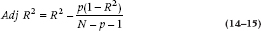
where p is the number of variables in the equation and N is the sample size. In Figure 14–5, we’ve plotted the Adj R² for various values of R² and p, assuming a sample size of 100. As you can see, there is less shrinkage as R² increases and as N is larger, but we pay a price for every variable we enter into the mix. You should also note that this equation produces less of a discrepancy between R² and Adj R² than most of the other equations, so the problem is probably worse than what the computer tells you.

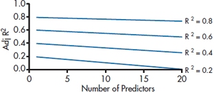
FIGURE 14-5 How adjusted R² is affected by R² and the number of predictor variables.

If you run a hierarchical or stepwise regression, you’ll see that, in the beginning, both R² and Adj R² increase with each variable entered (although, as expected, Adj R² won’t increase as much). Then, after a number of variables are in, R² will continue to increase slowly, but Adj R² will actually decrease. This indicates that the later variables are probably contributing more error than they’re accounting for.

INTERACTIONS

One simple addition to the armamentarium of the regressive (oops, regression) analyst is the incorporation of interaction terms in the regression equation. We have already described the glories of systematic use of interactions in Chapter 9, and the logic rubs off here as well.

As an example, there are several decades of research into the relationship between life stress and health. A predominant view is that the effect of stress is related to the accrual of several stressful events, such as divorce, a child leaving home,⁹ or a mortgage (Holmes, 1978). In turn, the model postulates that social supports can buffer or protect the individual from the vagaries of stress (Williams, Ware, and Donald, 1981). Imagine a study where we measured the number of stressful events and also the number of social relationships available, and now want to examine the relationship to doctor visits.¹⁰ The theory is really saying that, in the presence of more stressful events, more social supports will reduce the number of visits; in the presence of less stress, social supports are unrelated to visits. In short, an interaction exists between stress, social supports, and visits.

How do we incorporate this interaction in the model? Nothing could be simpler—we create a new variable by multiplying the stress and support variables. So, the equation is:

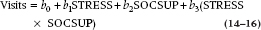
Finally, we would likely test the theory using hierarchical regression, where we would do one analysis with only the main effects and then a second analysis with the interaction term also, to see whether the interaction added significant prediction.

As you are no doubt painfully aware by this time, there ain’t no such thing as a free lunch; if something looks good, you have to pay a penalty somewhere. In this case, the cost of being able to look at interaction terms is the loss of power. Jaccard and Wan (1995) pointed out that the ability of an interaction to increase R² is related to the reliability, and that the reliability is the product of the reliabilities of the individual variables. So, if the scale measuring STRESS has a reliability of 0.80, and that tapping SOCSUP a reliability of 0.70, then the reliability of the interaction is 0.56, meaning that its effect on R² is just over half of what it would be if the reliability were 1.0.

DUMMY CODING

DO NOT SKIP THIS SECTION JUST BECAUSE YOU’RE SMART! We are not casting aspersions on the intelligence of people who code data; dummy coding refers to the way we deal with predictor variables that are measured on a nominal or ordinal scale. Multiple regression makes the assumption that the dependent variable is normally distributed, but it doesn’t make any such assumption about the predictors. However, we’d run into problems if we wanted to add a variable that captures that other aspect of “Yuppiness”—type of dwelling. If we coded Own Home = 1, Condo with Doorman = 2, and Other = 3, we would have a nominal variable. That is, we can change the coding scheme and not lose or gain any information. This means that treating DWELLING as if it were a continuous variable would lead to bizarre and misleading results; the b and β wouldn’t tell us how much Beemer Knee would increase as we moved from one type of dwelling to another, because we’d get completely different numbers with a different coding scheme.

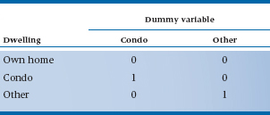
TABLE 14–8 Dummy coding for dwelling variable

The solution is breaking the variable down into a number of dummy variables. The rule is that if the original variable has k categories, we will make k − 1 dummies. In this case, because there are three categories, we will create two dummy variables. So, who gets left out in the cold? Actually, nobody. One of the categories is selected as the reference, against which the other categories are compared. Mathematically, it really doesn’t make much difference which one is chosen; usually it’s selected on logical or theoretical grounds. For example, if we had coded income into three levels (for Beemer owners, that would be 1 = $150,000 to $174,999; 2 = $175,000 to $199,999; and 3 = $200,000 and up¹¹), then it would make sense to have the paupers (Level 1) as the reference, and see to what degree greater income leads to more Beemer Knee. If there is no reason to choose one category over another (as is the case with DWELLING), it’s good practice to select the category with the largest number of subjects, because it will have the lowest standard error. Following Hardy (1993), the three guidelines for selecting the reference level are:

1. If you have an ordinal variable, choose either the upper or lower category.
   
2. Use a well-defined category; don’t use a residual one such as “Other.”
   
3. If you still have a choice, opt for the one with the largest sample size.

If we chose OWN HOME as the reference category, then the two dummy variables would be CONDO (with Doorman, naturally) and OTHER. Then, the coding scheme would look like Table 14–8; if a person lives in her own home, she would be coded 0 for both the CONDO and the OTHER dummy variables. A condo-dwelling person would be coded 1 for CONDO and 0 for OTHER; and someone who lives with his mother would be coded 0 for CONDO and 1 for OTHER.¹²

Now our regression equation is:

where b₆ tells us the increase or decrease in Beemer Knee for people who live in condos as compared with those who own a home, and b₇ does the same for the OTHER category as compared with OWN HOME.

The computer output will tell us whether b₆ and b₇ are significant, that is, different from the reference category. One question remains: How do we know if CONDO and OTHER are significantly different from each other? There are two ways to find out. The first method is rerunning the analysis, choosing a different category to be the reference. The second method is to get out our calculators and use some of the output from the computer program, namely, the variances and covariances of the regression coefficients. With these in hand, we can calculate a t-test:

where cov (b₆ b₇) means the covariance between the two bs.

WHAT’S LEFT OVER: LOOKING AT RESIDUALS

Let’s go back to the beginning for a moment. You’ll remember that our original equation looking at Beemer Knee was:

where the funny hat over the Y means that the equation is estimating the value of Y for each person. But, unless that equation results in perfect prediction (i.e., R and R² = 1, which occurs as often as sightings of polka-dotted unicorns), the estimate will be off for each individual to some degree. That means that each person will have two numbers representing the degree of Beemer Knee: Y, which is his or her actual value; and Yˆ, which is estimated value. The difference between the two, Y − Ŷ, is called the residual. Because the equation should overestimate Y as often as it underestimates it, the residuals should sum to zero, with some variance. Another way of defining R is that it’s the correlation between Y and Yˆ. When R = 1, Y and Yˆ are the same for every person; the lower the value of R, the more the values will deviate from one another, and the larger the residuals will be.

One of the assumptions of multiple regression is homoscedasticity, which means that the variance is the same at all points along the regression line. It’s a pain in the rear end if we had to calculate the variance at each value of the predictors, so we fall back on the granddaddy of all tests, the calibrated eyeball. Take a look at the left side of Figure 14–6, which shows a scatter plot for one predictor and one dependent variable, and the regression line. The points seem to be fairly evenly distributed above and below the line along its entire length. But, we can go a step further and look to see how the residuals are distributed. If we plot them against the predicted values, as we’ve done in the graph on the right side of Figure 14–6, the points should appear to be randomly placed above and below a value of 0, and no pattern should be apparent.

Now take a look at the left side of Figure 14–7. The data seem to fall above the regression line at low values of the predictor, then fall below the line, and then above it again—a situation called heteroscedasticity (i.e., not homoscedastic). This is even more apparent when we plot the residuals, as in the right side of the figure; they look like a double-jointed snake with scoliosis. This is only one of the patterns that shows up with heteroscedasticity. Sometimes the variance increases with larger values of the predictors, leading to the fan-shaped pattern, with the dots further from the line as we move from left to right. In brief, any deviation from a random scattering of points between ± 2 SDs is a warning that the data are heteroscedastic, and you may want to use one of the transformations outlined in Chapter 27 before going any further.

WHERE THINGS CAN GO WRONG

By now, you’re experienced enough in statistics to know that the issue is never, “Can things go wrong?” but, rather, “Where have things gone wrong?” However, before you can treat a problem, doctor, you have to know what’s wrong. So, we’re going to tell you what sorts of aches and pains a regression equation may come down with, and how to run all sorts of diagnostic tests to find out what the problem is.¹³ There are two main types of problems: those involving the cases (the specific disorders are discrepancy, leverage, and influence¹⁴) and those involving the variables (mainly multicollinearity).

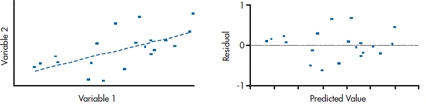
FIGURE 14-6 Scatter plot and plot of residuals when the data are homoscedastic.

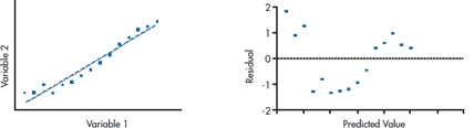
FIGURE 14-7 Scatter plot and plot of residuals when the data are heteroscedastic.

Discrepancy

The discrepancy, or distance, of a case is best thought of as the magnitude of its residual, that is, how much its predicted value of Y (Y-hat, or Ŷ) differs from the observed value. When the residual scores are standardized (as they usually are), then any value over 3.0 shows a subject whose residual is larger than that of 99% of the cases. The data for these outliers should be closely examined to see if there might have been a mistake made when recording or entering the data. If there isn’t an error you can spot, then you have a tough decision to make—to keep the case, or to trim it (which is a fancy way of saying “toss it out”). We’ll postpone this decision until we deal with “influence.”

Leverage

Leverage has nothing to do with junk bonds or Wall Street shenanigans. It refers to how atypical the pattern of predictor scores is for a given case. For example, it may not be unusual for a person to have a large number of clothes with designer labels; nor would it be unusual for a person to belong to no health clubs; but, in our sample, it would be quite unusual for a person to have a closet full of such clothes and not belong to health clubs. So, leverage relates to combinations of the predictor variables that are atypical for the group as a whole. Note that the dependent variable is not considered, only the independent variables.

A case that has a high leverage score has the potential to affect the regression line, but it doesn’t have to; we’ll see in a moment under what circumstances it will affect the line. Leverage for case i is often abbreviated as h_i, and it can range in value from 0 to (N − 1)/N, with a mean of p/N (where p is the number of predictors). Ideally, all of the cases should have similar values of h, which are close to p/N. Cases where h is greater than 2p/N should be looked on with suspicion.

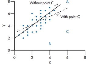
FIGURE 14-8 A depiction of cases with large values for leverage (Case A), discrepancy (Case B), and influence (Case C).

Influence

Now let’s put things together:

This means that distance and leverage individually may not influence the coefficients of the regression equation, but the two together may do so. Cases that have a large leverage score but are close to the regression line, and those that are far from the regression line but have small leverage scores, won’t have much influence; whereas cases that are high on both distance and leverage may exert a lot of influence. If you look at Figure 14–8, you’ll see what we mean. Case A is relatively far from the line (i.e., it’s discrepancy or distance is high), but the pattern of predictors (the leverage) is similar to that of the other cases. Case B has a high leverage score, but the discrepancy isn’t too great. Case C has the largest influence score, because it is relatively high on both indices. In fact, Case A doesn’t change the slope or intercept of the regression line at all, because it lies right on it (although it is quite distant from the other points). Case B, primarily because it is near the mean of X, has no effect on the slope, and lowers the value of the intercept just a bit. As you can see from the dashed regression line, Case C has an effect on (or “influences”) both the slope and the intercept.

Influence is usually indicated in computer outputs as “Cook’s distance,” or CD. CD measures how much the residuals of all of the other cases would change when a given case is deleted. A value over 1.00 shows that the subject’s scores are having an undue influence and it probably should be dropped.

Multicollinearity

Multiple regression is able to handle situations in which the predictors are correlated with each other to some degree. This is a good thing because, in most situations, it’s unusual for the “independent variables” to be completely independent from one another. Problems arise, however, when we cross the threshold from the undefined state of “to some degree” to the equally undefined state of “a lot.” We can often spot highly correlated variables just by looking at the correlation matrix. Multicollinearity refers to a more complex situation, in which the multiple correlation between one variable and a set of others is in the range of 0.90 or higher. This is much harder to spot, because the zero-order correlations among the variables may be relatively low, but the multiple correlation—which is what we’re concerned about—could be high. For example, if we measured a person’s height, weight, and body mass index (BMI), we’d find that they were all correlated with each other, but at an acceptable level. However, the multiple correlation of height and weight on the BMI would be well over 0.90.

Most computer programs check for this by calculating the squared multiple correlation (SMC, or R²) between each variable and all of the others. Some programs try to confuse us by converting the SMC into an index called tolerance,¹⁵ which is defined as (1 − R). The better programs test the SMC or tolerance of each variable, and kick out any that exceed some criterion (usually SMC ≥ 0.99, or tolerance ≤ 0.01). We would follow Tabachnick and Fidell’s (2001) advice to override this default and use a more stringent criterion. They recommend a maximum SMC of 0.90 (that is, a tolerance of 0.10), but Allison (1999) and others are even more conservative, advocating a maximum of 0.60, corresponding to a tolerance of 0.40. For once in our lives, we tend to side with the conservatives.

Yet another variant of the SMC that you’ll run across is the Variance Inflation Factor (VIF), which is the reciprocal of tolerance. For variable i:

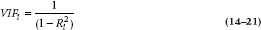
The main effect of multicollinearity is to inflate the values of the standard errors of the βs, which, in turn, drives them away from statistical significance. VIF is an index of how much the variance of the coefficients are inflated because of multicollinearity. More specifically, how much the standard error increases is given by the square root of the VIF; with a VIF of 9, the standard error is three times as large as it would be if the VIF were 1. This means that, in order to be significant, the coefficient would have to be three times larger. If we stick with our criterion that any R² over 0.90 indicates trouble, then any VIF over 10 means the same thing. Another effect of multicollinearity is the seemingly bizarre situation that some of the β weights have values greater than 1.0, which, in fact, can be used as a diagnostic test for the presence of multicollinearity.

Note that high multicollinearity doesn’t violate any of the assumptions of multiple regression. All of the estimates of the coefficients will be unbiased; it’s only the standard errors and confidence intervals that will be inflated and therefore the tests of significance underestimated.

There are a couple of situations that may result in multicollinearity in addition to high correlations among the predictors. One is screwing up dummy coding by not excluding one category. For example, if you divide marital status into six categories (Single, Married, Common-Law, Widowed, Divorced, and Separated) and used a dummy variable for each of them, you’ll run into problems. A second situation is including a variable that’s derived from other variables, and then including all of them. For instance, in some intelligence tests, the Full Scale IQ is in essence the mean of the Verbal and Performance IQs; if all three are included in a regression, you’ll get multicollinearity. Third, measuring the same variable twice but using different measures of it—for example, the prothrombin ratio and the International Normalized Ratio (INR)—will give you a severe case of the multicollinearities. Finally, you can run into problems if your regression equation includes a non-linear term, something we’ll discuss in Chapter 16. In essence, this means that we have a variable, such as Age, as well as Age². Since these two terms will be highly correlated, the result will be multicollinearity.

There are no easy ways to cure this malevolent condition. You should make sure you haven’t committed one of the errors we just mentioned regarding dummy coding or measuring the same thing twice. Another strategy is to increase the sample size, but that’s not always feasible. If you’ve thrown in a lot of variables just to see what’s going on, take them out (it was a bad idea to put them in to begin with). But dropping variables that make substantive sense just because they’re highly correlated with other variables is usually a bad practice; misspecification of the model is worse than multicollinearity. Finally, you can center the variables—something we discussed earlier in the chapter; this often reduces the correlations among them.

THE PRAGMATICS OF MULTIPLE REGRESSION

One real problem with multiple regression is that, as computers sprouted in every office, so did data bases, so now every damn fool with a lab coat has access to data bases galore. All successive admissions to the pediatric gerontology unit (both of them) are there in a data base. Score assigned to the personal interview for every applicant to the nursing school for the past 20 years, the 5% who came here and the 95% who went elsewhere or vanished altogether, are there in a data base. All the laboratory requisitions and routine tests ordered on the last 280,000 admissions to the hospital are there—in a data base.

A first level of response by any reasonable researcher to all this wealth of data and paucity of information should be, “Who cares?” But then, pressures to publish or perish being what they are, it seems that few can resist the opportunity to analyze them, usually without any previous good reason (i.e., hypothesis). Multiple regression is a natural for such nefarious tasks—all you need do is select a likely looking dependent variable (e.g., days to discharge from hospital, average class performance, undergraduate GPA—almost anything that seems a bit important), then press the button on the old “mult reg” machine, and stand back and watch the F-ratios fly. The last step is to examine all the significant coefficients (usually about 1 in 20), wax ecstatic about the theoretical reasons why a relationship might be so, and then inevitably recommend further research.

Given the potential for abuse, some checks and balances must exist to aid the unsuspecting reader of such tripe. Here are a few:

1. The number of data (patients, subjects, students) should be a minimum of 5 or 10 times the number of variables entered into the equation—not the number of variables that turn out to be significant, which is always small. Use the number you started with. This rule provides some assurance that the estimates are stable and not simply capitalizing on chance.
   
2. Inevitably, when folks are doing these types of post-hoc regressions, something significant will result. One handy way to see if it is any good is to simply square the multiple correlation. Any multiple regression worth its salt should account for about half the variance (i.e., a multiple R of about .7). Much less, and it’s not saying much.
   
3. Similarly, to examine the contribution of an individual variable before you start inventing a new theory, look at the change in R². This should be at least a few percent, or the variable is of no consequence in the prediction, statistically significant or not.
   
4. Look at the patterns in the regression equation. A gradual falloff should be seen in the prediction of each successive variable, so that variable 1 predicts, say, 20 to 30% of the variance, variable 2 an additional 10 to 15%, variable 3, 5 to 10% more, and so on, up to 5 or 6 variables and a total R² of .6 to .8. If all the variance is soaked up by the first variable, little of interest is found in the multiple regression. Conversely, if things dribble on forever, with each variable adding a little, it is about like number 2 above—not much happening here.
   
5. Remember that if you use one group of subjects to run the regression, you shouldn’t make definitive statements about the model using the same data. The real test is to see if the model applies in a new sample of people. If you have enough subjects, you should split the sample in two—run the regression with half of the subjects, and test it with the other half.

So these are some ways to deal with the plethora of multiple regressions out there. They reappear at the end of this section as C.R.A.P. Detectors, but we place them here to provide some sense of perspective.

SAMPLE SIZE CALCULATIONS

For once, nothing could be simpler. No one could possibly work out ahead of time what a reasonable value for a particular regression coefficient might be, let alone its SE. About all that can be hoped for is that the values that eventually emerge are reasonably stable and somewhere near the truth. The best guarantee of this is simply that the number of data be considerably more than the number of variables. Thus the “sample size calculation” is the essence of simplicity:

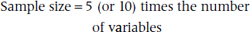
If you, or the reviewers of your grant, don’t believe us, try an authoritative source—Kleinbaum, Kupper, and Muller (1988).

Let’s point out why sample size is important. Strictly speaking, you can run a regression with as many subjects as predictors (i.e., variables and interaction terms). In fact, the results will look marvelous, with an R² value of 1.00 and many of the variables and interactions highly significant. This will be true even if all of the predictor variables are just random data. The model is over-fitted. The reason is that if we have 10 predictors and 10 subjects, we would in essence be estimating each β weight with a sample size of 1. Even doubling the number of subjects means that the sample size for each estimate is a whopping 2, not an ideal situation for ending up with a stable, replicable model. Also, the smaller the subject-to-variable ratio, the higher the rate of spurious R² values (Babyak, 2004). So, follow our advice—use at least 10 subjects per variable (and remember that each interaction term is another variable).

REPORTING GUIDELINES

Reporting the results of a multiple regression is a bit more complicated than for the tests we’ve described so far because there are usually two sets of findings we want to communicate: those for the individual variables, and those for the equation as a whole. Let’s start off with the former. What should be reported are:

Stay updated, free articles. Join our Telegram channel

Join