and Jordan Smoller2
(1)
Department of Epidemiology, Albert Einstein College of Medicine, Bronx, NY, USA
(2)
Department of Psychiatry and Center for Human Genetic Research, Massachusetts General Hospital, Boston, MA, USA
A statistician is someone who, with his head in an oven and his feet in a bucket of ice water, when asked how he feels, responds: “On the average, I feel fine.”
Anonymous
Different statistical techniques are appropriate depending on whether the variables of interest are discrete or continuous. We will first consider the case of discrete variables and present the chi-square test, and then we will discuss methods applicable to continuous variables.
3.1 Chi-Square for 2 × 2 Tables
The chi-square test is a statistical method to determine whether the results of an experiment may arise by chance or not. Let us, therefore, consider the example of testing an anticoagulant drug on female patients with myocardial infarction. We hope the drug lowers mortality, but we set up our null hypothesis as follows:
♦ Null hypothesis
There is no difference in mortality between the treated group of patients and the control group
♦ Alternate hypothesis
The mortality in the treated group is lower than in the control group
(The data for our example come from a study done a long time ago and refer to a specific high-risk group.8 They are used for illustrative purposes, and they do not reflect current mortality rates for people with myocardial infarction.)
We then record our data in a 2 × 2 contingency table in which each patient is classified as belonging to one of the four cells:

Observed frequencies

The mortality in the control group is 40/129 = 31 % and in the treated it is 39/262 = 15 %. But could this difference have arisen by chance? We use the chi-square test to answer this question. What we are really asking is whether the two categories of classification (control vs. treated by lived vs. died) are independent of each other. If they are independent, what frequencies would we expect in each of the cells? And how different are our observed frequencies from the expected ones? How do we measure the size of the difference?
To determine the expected frequencies, consider the following:


If the categories are independent, then the probability of a patient being both a control and living is P(control) × P(lived). [Here we apply the law referred to in chapter 2 on the joint probability of two independent events.]
The expected frequency of an event is equal to the probability of the event times the number of trials = N × P. So the expected number of patients who are both controls and live is
![$$ \begin{array}{c}\hfill N\times P\left( control\; and\; lived\right)=N\times P(control)\times P(lived)\hfill \\ {}\hfill =N\left[\frac{\left(a+c\right)}{N}\times \frac{\left(a+b\right)}{N}\right]=\left(a+c\right)\times \frac{\left(a+b\right)}{N}\hfill \end{array} $$](/wp-content/uploads/2016/11/A270404_4_En_3_Chapter_Equa.gif)
![$$ \begin{array}{c}\hfill N\times P\left( control\; and\; lived\right)=N\times P(control)\times P(lived)\hfill \\ {}\hfill =N\left[\frac{\left(a+c\right)}{N}\times \frac{\left(a+b\right)}{N}\right]=\left(a+c\right)\times \frac{\left(a+b\right)}{N}\hfill \end{array} $$](/wp-content/uploads/2016/11/A270404_4_En_3_Chapter_Equa.gif)
In our case, this yields the following table:


Another way of looking at this is to say that since 80 % of the patients in the total study lived (i.e., 312/391 = 80 %), we would expect that 80 % of the control patients and 80 % of the treated patients would live. These expectations differ, as we see, from the observed frequencies noted earlier, that is, those patients treated did, in fact, have a lower mortality than those in the control group.
Well, now that we have a table of observed frequencies and a table of expected values, how do we know just how different they are? Do they differ just by chance or is there some other factor that causes them to differ? To determine this, we calculate a value called chi-square (also written as  2). This is obtained by taking the observed value in each cell, subtracting from it the expected value in each cell, squaring this difference, and dividing by the expected value for each cell. When this is done for each cell, the four resulting quantities are added together to give a number called chi-square. Symbolically this formula is as follows:
 where O is the observed frequency and e is the expected frequency in each cell.
 2). This is obtained by taking the observed value in each cell, subtracting from it the expected value in each cell, squaring this difference, and dividing by the expected value for each cell. When this is done for each cell, the four resulting quantities are added together to give a number called chi-square. Symbolically this formula is as follows:
This number, called chi-square, is a statistic that has a known distribution. What that means, in essence, is that for an infinite number of such 2 × 2 tables, chi-squares have been calculated, and we thus know what the probability is of getting certain values of chi-square. Thus, when we calculate a chi-square for a particular 2 × 2 contingency table, we know how likely it is that we could have obtained a value as large as the one that we actually obtained strictly by chance, under the assumption the hypothesis of independence is the correct one, that is, if the two categories of classification were unrelated to one another or if the null hypothesis were true. The particular value of chi-square that we get for our example happens to be 13.94.
From our knowledge of the distribution of values of chi-square, we know that if our null hypothesis is true, that is, if there is no difference in mortality between the control and treated group, then the probability that we get a value of chi-square as large or larger than 13.94 by chance alone is very, very low; in fact this probability is less than .005. Since it is not likely that we would get such a large value of chi-square by chance under the assumption of our null hypothesis, it must be that it has arisen not by chance but because our null hypothesis is incorrect. We, therefore, reject the null hypothesis at the .005 level of significance and accept the alternate hypothesis, that is, we conclude that among women with myocardial infarction, the new drug does reduce mortality. The probability of obtaining these results by chance alone is less than 5/1000 (.005). Therefore, the probability of rejecting the null hypothesis, when it is in fact true (type I error) is less than .005.
The probabilities for obtaining various values of chi-square are tabled in most standard statistics texts, so that the procedure is to calculate the value of chi-square and then look it up in the table to determine whether or not it is significant. That value of chi-square that must be obtained from the data in order to be significant is called the critical value. The critical value of chi-square at the .05 level of significance for a 2 × 2 table is 3.84. This means that when we get a value of 3.84 or greater from a 2 × 2 table, we can say there is a significant difference between the two groups. Appendix 1 provides some critical values for chi-square and for other tests.
In actual usage, a correction is applied for 2 × 2 tables known as the Yates’ correction and calculation is done using the formula
![$$ \frac{N{\left[\left| ad-bc\right|-\frac{N}{2}\right]}^2}{\left(a+b\right)\left(c+d\right)\left(a+c\right)\left(b+d\right)} $$](/wp-content/uploads/2016/11/A270404_4_En_3_Chapter_Equc.gif)
![$$ \frac{N{\left[\left| ad-bc\right|-\frac{N}{2}\right]}^2}{\left(a+b\right)\left(c+d\right)\left(a+c\right)\left(b+d\right)} $$](/wp-content/uploads/2016/11/A270404_4_En_3_Chapter_Equc.gif)
Note: |ad–bc| means the absolute value of the difference between a × d and b × c. In other words, if a × d is greater than b × c, subtract bc from ad; if bc is greater than ad, subtract ad from bc. The corrected chi-square so calculated is 12.95, still well above the 3.84 required for significance.
The chi-square test should not be used if the numbers in the cells are too small. The rules of thumb: When the total N is greater than 40, use the chi-square test with Yates’ correction. When N is between 20 and 40 and the expected frequency in each of the four cells is 5 or more, use the corrected chi-square test. If the smallest expected frequency is less than 5, or if N is less than 20, use the Fisher’s test.
While the chi-square test approximates the probability, the Fisher’s exact test gives the exact probability of getting a table with values like those obtained or even more extreme. A sample calculation is shown in Appendix 2. The calculations are unwieldy, but the Fisher’s exact test is also usually included in most statistics programs for personal computers. More on this topic may be found in the book Statistical Methods for Rates and Proportions by Joseph L. Fleiss. The important thing is to know when the chi-square test is or is not appropriate.
3.2 McNemar Test
Suppose we have the situation where measurements are made on the same group of people before and after some intervention, or suppose we are interested in the agreement between two judges who evaluate the same group of patients on some characteristics. In such situations, the before and after measures, or the opinions of two judges, are not independent of each other, since they pertain to the same individuals. Therefore, the chi-square test or the Fisher’s exact test is not appropriate. Instead, we can use the McNemar test.
Consider the following example. Case histories of patients who were suspected of having ischemic heart disease (a decreased blood flow to the heart because of clogging of the arteries) were presented to two cardiology experts. The doctors were asked to render an opinion on the basis of the available information about the patient. They could recommend either (1) that the patient should be on medical therapy or (2) that the patient have an angiogram, which is an invasive test, to determine if the patient is a suitable candidate for coronary artery bypass graft surgery (known as CABG). Table 3.1 shows the results of these judgments on 661 patients.
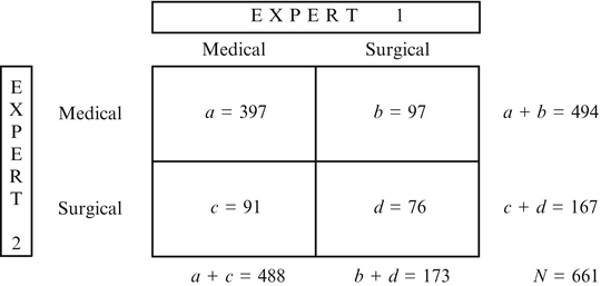
Table 3.1

Note that in cell b Expert 1 advised surgery and Expert 2 advised medical therapy for 97 patients, whereas in cell c Expert 1 advised medical therapy and Expert 2 advised surgery for 91 of the patients. Thus, the two physicians disagree in 188 of the 661 cases or 28 % of the time. Cells a and d represent patients about whom the two doctors agree. They agree in 473 out the 661 case or 72 % of the time.
To determine whether the observed disagreement could have arisen by chance alone under the null hypothesis of no real disagreement in recommendations between the two experts, we calculate a type of chi-square value as follows:
 (|b–c| means the absolute value of the difference between the two cells, that is, irrespective of the sign; the −1 in the numerator is analogous to the Yates’ correction for chi-square described in Section 3.1 and gives a better approximation to the chi-square distribution.) A chi-square of .13 does not reach the critical value of chi-square of 3.84 needed for a .05 significance level, as described in Section 3.1, so we cannot reject the null hypothesis, and we conclude that our data are consistent with no difference in the opinions of the two experts. Were the chi-square test significant, we would have to reject the null hypothesis and say the experts significantly disagree. However, such a test does not tell us about the strength of their agreement, which can be evaluated by a statistic called Kappa.

3.3 Kappa
The two experts could be agreeing just by chance alone, since both experts are more likely to recommend medical therapy for these patients. Kappa is a statistic that tells us the extent of the agreement between the two experts above and beyond chance agreement.


To calculate the expected number of cases in each cell of the table, we follow the procedure described for chi-square in Section 3.1. The cells a and d in Table 3.1 represent agreement. The expected number by chance alone is
 So the proportion of agreement expected by chance alone is


that is, by chance alone, the experts would be expected to agree 62 % of the time. The proportion of observed agreement is
 If the two experts agreed at the level of chance only, Kappa would be 0; if the two experts agreed perfectly, Kappa would be 1.

3.4 Description of a Population: Use of the Standard Deviation
In the case of continuous variables, as for discrete variables, we may be interested in description or in inference. When we wish to describe a population with regard to some characteristic, we generally use the mean or average as an index of central tendency of the data.
Other measures of central tendency are the median and the mode. The median is that value above which 50 % of the other values lie and below which 50 % of the values lie. It is the middle value or the 50th percentile. To find the median of a set of scores, we arrange them in ascending (or descending) order and locate the middle value if there are an odd number of scores, or the average between the two middle scores if there are an even number of scores. The mode is the value that occurs with the greatest frequency. There may be several modes in a set of scores but only one median and one mean value. These definitions are illustrated below. The mean is the measure of central tendency most often used in inferential statistics.
Measures of central tendency | |
|---|---|
Set of scores | Ordered |
12 | 6 |
12 | 8 |
6 | 10 |
8 | 11 Median |
11 | 12 Mode |
10 | 12 |
15 | 15 |
SUM: 74 | Mean = 74/7 = 10.6 |
The true mean of the population is called m, and we estimate that mean from data obtained from a sample of the population. The sample mean is called  (read as x bar). We must be careful to specify exactly the population from which we take a sample. For instance, in the general population, the average IQ is 100, but the average IQ of the population of children age 6–11 years whose fathers are college graduates is 112.9 Therefore, if we take a sample from either of these populations, we would be estimating a different population mean, and we must specify to which population we are making inferences.
 (read as x bar). We must be careful to specify exactly the population from which we take a sample. For instance, in the general population, the average IQ is 100, but the average IQ of the population of children age 6–11 years whose fathers are college graduates is 112.9 Therefore, if we take a sample from either of these populations, we would be estimating a different population mean, and we must specify to which population we are making inferences.
However, the mean does not provide an adequate description of a population. What is also needed is some measure of variability of the data around the mean. Two groups can have the same mean but be very different. For instance, consider a hypothetical group of children each of whose individual IQ is 100; thus, the mean is 100. Compare this to another group whose mean is also 100 but includes individuals with IQs of 60 and those with IQs of 140. Different statements must be made about these two groups: one is composed of all average individuals and the other includes both retardates and geniuses.
The most commonly used index of variability is the standard deviation (s.d.), which is a type of measure related to the average distance of the scores from their mean value. The square of the standard deviation is called variance. The population standard deviation is denoted by the Greek letter σ (sigma). When it is calculated from a sample, it is written as s.d. and is illustrated in the example below:
 (In Group A since each score is equal to the mean of 100, there are no deviations from the mean of A.)
 An equivalent formula for s.d. that is more suited for actual calculations is

IQ scores | Deviations from mean | Squared scores for B | ||
|---|---|---|---|---|
Group A | Group B |  |  | x b 2 |
100 | 60 | −40 | 1,600 | 3,600 |
100 | 140 | 40 | 1,600 | 19,600 |
100 | 80 | −20 | 400 | 6,400 |
100 | 120 | 20 | 400 | 14,400 |
 |  | Σ = 0 | Σ = 4,000 of squared deviations | Σ = 44,000 sum of squares |


For group B we have
 Variance = (s.d.)2

Note the mean of both groups is 100, but the standard deviation of group A is 0, while the s.d. of group B is 36.51. (We divide the squared deviations by n–1 rather than by n because we are estimating the population σ from sample data, and dividing by n–1 gives a better estimate. The mathematical reason is complex and beyond the scope of this book.)
3.5 Meaning of the Standard Deviation: The Normal Distribution
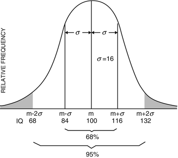
The standard deviation is a measure of the dispersion or spread of the data. Consider a variable like IQ, which is normally distributed, that is, it can be described by the familiar, bell-shaped curve where most of the values fall around the mean with decreasing number of values at either extremes. In such a case, 68 % of the values lie within 1 standard deviation on either side of the mean, 95 % of the values lie within 2 standard deviations of the mean, and 99 % of the values lie within 3 standard deviations of the mean. (The IQ test was originally constructed so that it had a mean of 100 and a standard deviation of 16.)
In the population at large, 95 % of people have IQs between 68 and 132. Approximately 2.5 % of people have IQs above 132 and another 2.5 % of people have IQs below 68. (This is indicated by the shaded areas at the tails of the curves.)
If we are estimating from a sample and if there are a large number of observations, the standard deviation can be estimated from the range of the data, that is, the difference between the smallest and the highest value. Dividing the range by 6 provides a rough estimate of the standard deviation if the distribution is normal, because 6 standard deviations (3 on either side of the mean) encompass 99 %, or virtually all, of the data.
On an individual, clinical level, knowledge of the standard deviation is very useful in deciding whether a laboratory finding is normal, in the sense of “healthy.” Generally a value that is more than 2 standard deviations away from the mean is suspect, and perhaps further tests need to be carried out.
For instance, suppose as a physician you are faced with an adult male who has a hematocrit reading of 39. Hematocrit is a measure of the amount of packed red cells in a measured amount of blood. A low hematocrit may imply anemia, which in turn may imply a more serious condition. You also know that the average hematocrit reading for adult males is 47. Do you know whether the patient with a reading of 39 is normal (in the sense of health) or abnormal? You need to know the standard deviation of the distribution of hematocrits in people before you can determine whether 39 is a normal value. In point of fact, the standard deviation is approximately 3.5; thus, plus or minus 2 standard deviations around the mean results in the range of from 40 to 54 so that 39 would be slightly low. For adult females, the mean hematocrit is 42 with a standard deviation of 2.5, so that the range of plus or minus 2 standard deviations away from the mean is from 37 to 47. Thus, if an adult female came to you with a hematocrit reading of 39, she would be considered in the “normal” range.
3.6 The Difference Between Standard Deviation and Standard Error
Often data in the literature are reported as ± s.d. (read as mean + or −1 standard deviation). Other times they are reported as ± s.e. (read as mean + or −1 standard error). Standard error and standard deviation are often confused, but they serve quite different functions. To understand the concept of standard error, you must remember that the purpose of statistics is to draw inferences from samples of data to the population from which these samples came. Specifically, we are interested in estimating the true mean of a population for which we have a sample mean based on, say, 25 cases. Imagine the following:
Population IQ scores, x i | Sample means based on 25 people randomly selected | |
|---|---|---|
110 |  | |
100 | ||
105 |  | |
98 | ||
140 |  | |
– |  | |
– | – | |
100 | 100 | |
m = mean of all the x i s |  , mean of the means is m, the population mean , mean of the means is m, the population mean | |
σ = population standard deviation |  Standard deviation of the distribution of the Standard deviation of the distribution of the  called the standard error of the mean = called the standard error of the mean =  | |
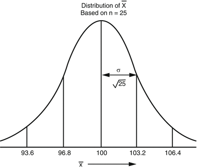
There is a population of IQ scores whose mean is 100 and its standard deviation is 16. Now imagine that we draw a sample of 25 people at random from that population and calculate the sample mean  . This sample mean happens to be 102. If we took another sample of 25 individuals, we would probably get a slightly different sample mean, for example, 99. Suppose we did this repeatedly an infinite (or a very large) number of times, each time throwing the sample, we just drew back into the population pool from which we would sample 25 people again. We would then have a very large number of such sample means. These sample means would form a normal distribution. Some of them would be very close to the true population mean of 100, and some would be at either end of this “distribution of means” as in Figure 3.2.
 . This sample mean happens to be 102. If we took another sample of 25 individuals, we would probably get a slightly different sample mean, for example, 99. Suppose we did this repeatedly an infinite (or a very large) number of times, each time throwing the sample, we just drew back into the population pool from which we would sample 25 people again. We would then have a very large number of such sample means. These sample means would form a normal distribution. Some of them would be very close to the true population mean of 100, and some would be at either end of this “distribution of means” as in Figure 3.2.
Figure 3.2
Distribution of sample means
This distribution of sample means would have its own standard deviation, that is, a measure of the spread of the data around the mean of the data. In this case, the data are sample means rather than individual values. The standard deviation of this distribution of means is called the standard error of the mean.
It should be pointed out that this distribution of means, which is also called the sampling distribution of means, is a theoretical construct. Obviously, we don’t go around measuring samples of the population to construct such a distribution. Usually, in fact, we just take one sample of 25 people and imagine what this distribution might be. However, due to certain mathematical derivations, we know a lot about this theoretical distribution of population means, and therefore we can draw important inferences based on just one sample mean. What we do know is that the distribution of means is a normal distribution, that its mean is the same as the population mean of the individual values, that is, the mean of the means is m, and that its standard deviation is equal to the standard deviation of the original individual values divided by the square root of the number of people in the sample.
Standard error of the mean =


In this case it would be


The distribution of means would look as shown in Figure 3.2.
Please note that when we talk about population values, which we usually don’t know but are trying to estimate, we refer to the mean as m and the standard deviation as σ. When we talk about values calculated from samples, we refer to the mean as  , the standard deviation as s.d., and the standard error as s.e.
 , the standard deviation as s.d., and the standard error as s.e.
Now imagine that we have a distribution of means based on samples of 64 individuals. The mean of these means is also m, but its dispersion, or standard error, is smaller. It is  . This is illustrated in Figure 3.3.
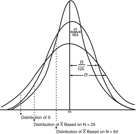
 . This is illustrated in Figure 3.3.
Figure 3.3
Distribution of means for different sample sizes
It is easily seen that if we take a sample of 25 individuals, their mean is likely to be closer to the true mean than the value of a single individual, and if we draw a sample of 64 individuals, their mean is likely to be even closer to the true mean than was the mean we obtained from the sample of 25. Thus, the larger the sample size, the better is our estimate of the true population mean.
The standard deviation is used to describe the dispersion or variability of the scores. The standard error is used to draw inferences about the population mean from which we have a sample. We draw such inferences by constructing confidence intervals, which are discussed in Section 3.11.
3.7 Standard Error of the Difference Between Two Means
This concept is analogous to the concept of standard error of the mean. The standard error of the differences between two means is the standard deviation of a theoretical distribution of differences between two means. Imagine a group of men and a group of women each of whom have an IQ measurement. Suppose we take a sample of 64 men and a sample of 64 women, calculate the mean IQs of these two samples, and obtain their differences. If we were to do this an infinite number of times, we would get a distribution of differences between sample means of two groups of 64 each. These difference scores would be normally distributed; their mean would be the true average difference between the populations of men and women (which we are trying to infer from the samples), and the standard deviation of this distribution is called the standard error of the differences between two means.
The standard error of the difference between two means of populations X and Y is given by the formula
 where σ x 2 is the variance of population X and σ y 2 is the variance of population Y, n x is the number of cases in the sample from population X and n y , is the number of cases in the sample from population Y.

In some cases, we know or assume that the variances of the two populations are equal to each other and that the variances that we calculate from the samples we have drawn are both estimates of a common variance. In such a situation, we would want to pool these estimates to get a better estimate of the common variance. We denote this pooled estimate as s pooled2 = s p 2, and we calculate the standard error of the difference between means as
 We calculate s p 2 from sample data:


This is the equivalent to


Since in practice we will always be calculating our values from sample data, we will henceforth use the symbology appropriate to that.
3.8 Z Scores and the Standardized Normal Distribution
The standardized normal distribution is one whose mean = 0, standard deviation = 1, and the total area under the curve = 1. The standard normal distribution looks like the one shown in Figure 3.4.
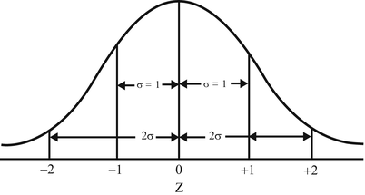

Figure 3.4
Standard normal distribution
On the abscissa, instead of x, we have a transformation of x called the standard score; Z. Z is derived from x by the following:
 Thus, the Z score really tells you how many standard deviations from the mean a particular x score is.

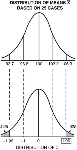
Any distribution of a normal variable can be transformed to a distribution of Z by taking each x value, subtracting from it the mean of x (i.e., m), and dividing this deviation of x from its mean, by the standard deviation. Let us look at the IQ distribution again in Figure 3.5.
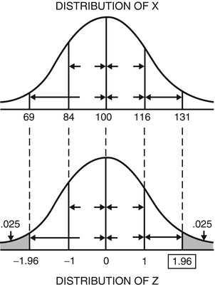

Figure 3.5
Distribution of Z scores
Thus, an IQ score of 131 is equivalent to a Z score of 1.96 (i.e., it is 1.96, or nearly 2, standard deviations above the mean IQ).


One of the nice things about the Z distribution is that the probability of a value being anywhere between two points is equal to the area under the curve between those two points. (Accept this on faith.) It happens that the area to the left of 1.96 corresponds to a probability of .025, or 2.5 % of the total curve. Since the curve is symmetrical, the probability of Z being to the left of −1.96 is also .025. Invoking the additive law of probability (Section 2.2), the probability of a Z being either to the left of −1.96 or to the left of +1.96 is .025 + .025 = .05. Transforming back up to x, we can say that the probability of someone having an IQ outside of 1.96 standard deviations away from the mean (i.e., above 131 or below 69) is .05, or only 5 % of the population have values that extreme. (Commonly, the Z value of 1.96 is rounded off to ±2 standard deviations from the mean as corresponding to the cutoff points beyond which lies 5 % of the curve, but the accurate value is 1.96.)
A very important use of Z derives from the fact that we can also convert a sample mean (rather than just a single individual value) to a Z score.
 The numerator now is the distance of the sample mean from the population mean, and the denominator is the standard deviation of the distribution of means, which is the standard error of the mean. This is illustrated in Figure 3.6, where we are considering means based on 25 cases each. The s.e. is
  .
.

 .
.
