6.1 How Does Natural Selection Work?

A common approach to natural selection in biology classes is to simulate the process using laboratory organisms such as fruit flies, whose short generation lengths make them amenable to observing evolution over short periods of time. Natural selection can also be modeled using simple mathematics, an approach that provides many insights into how natural selection can operate in nature.

6.1.1 Absolute and Relative Fitness

As noted above, the term fitness goes beyond any simple equation with physical fitness. When modeling natural selection, fitness simply refers to the probability of survival and reproduction. Models of natural selection are based on each genotype being associated with a specific fitness, which expresses the relative probability of representation in the next generation. This might sound rather abstract, but a simple example shows how this works.

We start with our standard model of a locus with two alleles, A and a, such that we have three genotypes: AA, Aa, and aa. Imagine that we have the following numbers of individuals in a population at birth: 500 individuals with genotype AA, 1000 with genotype Aa, and 500 with genotype aa, for a total of 2000 individuals. Imagine that we examine this population later in time to see how many have survived to reproductive age, and find that there are now 1575 individuals made up of 450 with genotype AA, 900 with genotype Aa, and 225 with genotype aa. We now compare the number of each genotype for the 2 times in the following table:

We can see that there has been some mortality; of the original 2000 individuals, 1575 survived to adulthood and 425 did not. However, if we look more closely, we see that this mortality was not the same for each genotype. Our interest is in the proportional change for each genotype, which is known as absolute fitness, which can be computed for each genotype by taking the ratio of the numbers at two points in time, which gives

AA	Aa	aa

We can now easily see that although some individuals from each genotype did not survive, this mortality was not the same for all genotypes. Proportionally, far more individuals died that had genotype aa than was the case for genotypes AA or Aa. In this example, we considered only differential mortality, but we can also consider similar effects from differential fertility, where there are differences in the number of births by genotype.

Mathematically, it is easier to deal with a quantity known as relative fitness, which expresses fitness relative to the most fit genotype. Relative fitness is typically denoted by the letter w, with subscripts used to refer to the different genotypes. Thus, the symbol wAA is used to refer to the relative fitness of genotype AA, wAa is used to refer to the relative fitness of genotype Aa, and waa is used to refer to the relative fitness of genotype aa. These values are easily computed by dividing each absolute fitness value by the highest absolute fitness value, which sets the highest relative fitness equal to 1 by definition. In terms of the example above, the highest absolute fitness, shared by both genotypes AA and Aa, is 0.9, which means that the relative fitness values are

AA	Aa	aa

In relative terms, these numbers mean that for every 100 individuals with genotype AA (or Aa) that survive, only 50 with genotype aa survive. This type of variation in fitness is typical of a recessive allele that is harmful when two copies are inherited (the homozygous genotype aa), but not when only one copy is inherited (the heterozygous genotype Aa).

If the absolute fitness of all three genotypes were the same, then all of the relative fitness values would also be the same, and all would equal 1.0. In this case, there would be no differential survival and/or reproduction by genotype, and allele frequencies would remain at Hardy–Weinberg equilibrium. If at least one fitness value differed among the three genotypes, then natural selection would occur. Natural selection can sometimes cause an allele to increase in frequency, sometimes decrease in frequency, and sometimes reach a balance. The specific effect of natural selection depends on the fitness of each specific genotype. Several examples of likely forms of natural selection will be described later in this chapter.

6.1.2 A Simulation of Natural Selection

At this point, we will relate the concept of relative fitness to natural selection by means of a simple mathematical simulation that uses some of the basic rules of probability outlined in Chapter 1. This simulation will use the standard model of a locus with two alleles, A and a. In order to simulate the process, we need the initial allele frequencies (p and q) and the relative fitness of each genotype: wAA, wAa, and waa. For this example, we will start with allele frequencies of p = 0.5 and q = 0.5 and relative fitness values of: wAA = 1.0, wAa = 1.0, and waa = 0.5.

6.1.2.1 Step 1: Start with Genotype Frequencies under Hardy–Weinberg Equilibrium

We start off by determining the expected genotype frequencies of the population before selection by deriving the Hardy–Weinberg proportions. Given p = 0.5 and q = 0.5, these are

6.1.2.2 Step 2: Compute Change in Genotype Frequencies Due to Selection

If there were no selection, the proportions above would also be the expected proportions in the next generation. Under selection, however, we need to model differential fitness. First, we list the fitness values under their respective genotypes:

Each row here represents probabilities associated with each genotype. The first row (before selection) shows the probabilities of having a given genotype. The second row (fitness) shows the probabilities that someone with a given genotype will contribute genetically to the next generation. Therefore, the probability that someone has a given genotype AND contributes genetically to the next generation is solved using the AND rule, which entails multiplying these probabilities. The expected genotype proportions after selection are therefore obtained as follows:

An important quantity is the sum of the genotype frequencies after selection:

This number is the mean fitness across the three genotypes (denoted w ). The mean fitness is not simply the average of the three relative fitness values, which would be = [(1 + 1 + 0.5)/3], but instead is a mean where each relative fitness is weighted by the frequency of that genotype in the population after selection. The mean fitness tells us how much selection has taken place relative to the case where no selection has occurred (where the mean fitness under Hardy–Weinberg equilibrium would be equal to 1.0). Here, the mean fitness of 0.875 means that 87.5% of the individuals survive, and therefore that 100 − 87.5 = 12.5% did not survive.

6.1.2.3 Step 3: Normalize Genotype Frequencies

What effect do you think selection has had on the allele frequencies? It may seem intuitive that the frequency of the a allele will decrease because we are selecting out half of those individuals with the aa genotype. This is correct, but to see the exact effect, we need to compute the allele frequencies after selection. Although we usually compute allele frequencies from genotype frequencies using equation 2.3, where we add the frequency of one homozygote to half the frequency of the heterozygote, we cannot do so in this case because the genotype frequencies after selection do not add up to 1.0. Instead, they add up to the mean fitness. To circumvent this problem, we need to express the genotype frequencies after selection relative to the mean fitness, which is easily done by dividing each genotype frequency by the mean fitness. This process is called normalization. After doing this, our table has a new row and looks like this:

Note that the sum of the normalized genotype frequencies now adds up to 1.0 (0.2857 + 0.5714 + 0.1429 = 1.0).

6.1.2.4 Step 4: Compute New Allele Frequencies

Given the normalized genotype frequencies after selection, we can now compute the new allele frequencies using equation 2.3:

We can easily see the impact of natural selection after a single generation. Here, the frequency of the a allele has decreased as expected, from q = 0.5 to 0.4286. Because the frequency of q decreases, the frequency of p increases, from 0.5 to 0.5714.

When we begin to track changes in allele frequencies due to selection over many generations, it will be useful to keep track of the exact amount of change from one generation to the next. If we refer to p and q as the allele frequencies before selection and the symbols p′ and q′ as the allele frequencies after selection, then the amount of change in a given generation (Δ) will be equal to

The value for Δp is positive because the A allele increased in frequency, and the value for Δq is negative because the a allele decreased in frequency.

6.1.2.5 Step 5: Extend the Results to the Next Generation

We can now repeat steps 1–4 by taking the new allele frequencies (p = 0.5714 and q = 0.4286) and starting over and the assuming that the fitness values remain the same. Filling in all the rows of the table that we built, we now obtain

Finally, after selection, the new values of p and q after the second generation of selection are p = 0.6292 and q = 0.3708, respectively. The frequency of the a allele has continued to decrease, and Δq now equals 0.3708 − 0.4286 = − 0.0578. The mean fitness (the sum of the unnormalized genotype frequencies after selection) has increased from 0.875 in the first generation to

in the second generation. This increase is due to the reduction in individuals susceptible to selection (those with genotype aa in this particular example).

The above process can be repeated generation after generation. Although the computations could be done by hand, they would become rather tiresome quickly, and it is much easier to use a spreadsheet program. Using such a program, I simulated 100 generations of selection. The results are shown in Figures 6.1, 6.2, 6.3. Figure 6.1 shows how the frequency of the a allele (q) decreases over time because of selection against individuals with genotype aa. This decrease is rapid at first, and then slows down because there are proportionately fewer individuals with genotype aa to select against each generation.

Figure 6.1 Allele frequency under selection against the recessive homozygote. Initial allele frequencies are p = 0.5 and q = 0.5. Fitness values are wAA = 1.0, wAa = 1.0, and waa = 0.5. The frequency of the a allele (q) decreases over time; the decrease is rapid at first and then slows down. Over time, the frequency of q will approach zero.

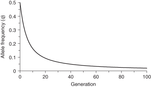
Figure 6.2 Allele frequency change per generation under selection against the recessive homozygote. Initial allele frequencies are p = 0.5 and q = 0.5. Fitness values are wAA = 1.0, wAa = 1.0, and waa = 0.5. With each generation the amount of change is negative because the allele frequency q is decreasing over time (see Figure 6.1). Over time, the amount of change approaches zero.

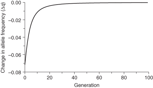
Figure 6.3 Mean fitness in each generation under selection against the recessive homozygote. Initial allele frequencies are p = 0.5 and q = 0.5. Fitness values are wAA = 1.0, wAa = 1.0, and waa = 0.5. Mean fitness increases with each generation, rapidly at first and then slowing down to approach a maximum value of 1.

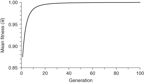
Figure 6.2 shows the amount of allele frequency change per generation (Δq). The amount of change is negative from one generation to the next, because the frequency of q decreases over time. However, the magnitude of this change decreases over time as the impact of selection declines with fewer aa individuals. Thus, Δq approaches a value of zero, which is at equilibrium when q = 0 and there will be no further change. In a mathematical sense, q will never reach 0 but will approach it. In a practical sense, there will come a point where q is so low that it becomes zero because of genetic drift.

Figure 6.3 shows how mean fitness increases over time to approach a theoretical maximum where p = 1, q = 0, and the mean fitness = 1. This graph is important in understanding natural selection, because it is a process that leads, generation after generation, toward maximizing mean fitness.

6.2 A General Model of Natural Selection

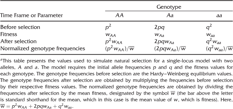
In order to simulate any case of selection for a single locus with two alleles, we need the initial allele frequencies and the relative fitness for each genotype. We then can take the tables presented in the five-step example above and substitute the appropriate mathematical variables for the specific values used in the example. Table 6.1 shows the expected genotype frequencies before selection (obtained from Hardy–Weinberg equilibrium), the genotype frequencies after selection, and the normalized genotype frequencies after selection. The formulas presented in Table 6.1 are used for deriving several quantities below. The derivations presented in this chapter are taken from Ayala (1982).

Table 6.1 A General Model of Natural Selectiona

The first quantity that we derive (and that is needed to compute the normalized genotype frequencies) is the mean fitness, computed as the sum of the genotype frequencies after selection:

6.1

We now derive the allele frequencies after a single generation of selection, labeled as p′ and q′, by using equation 2.3 on the appropriate normalized genotype frequencies after selection from Table 6.1. For p′, this gives

from equation 2.3, which, when used with the values in Table 6.1, gives

We then factor out p to get

6.2

We do the same thing for q′ to obtain

6.3

(Note: To follow this, be sure to keep the subscripts for the fitness values straight!) We could then solve for additional generations by setting the initial allele frequencies equal to p′ and q′ and solving for the next generation (again, assuming that the fitness values do not change).

We are also interested in the amount of change in allele frequencies: Δp and Δq. Derivation of these values is a bit more involved algebraically, and is presented in Appendix 6.6. These values are

6.4

and

6.5

6.3 Types of Natural Selection

Given the general model above, we will use equations (6.1)–(6.5) to explore several common types of natural selection.

6.3.1 Selection against the Recessive Homozygote

The worked example of natural selection given earlier (Figures 6.1, 6.2, 6.3) involved selection against the recessive homozygote. This type of selection is common with a number of genetic disorders where having two copies of a harmful recessive allele lowers an individual’s fitness. In the most extreme case, that of a lethal recessive, the fitness is zero. The general model of natural selection can be used to explore some general implications of selection against the recessive homozygote. Here, we use our standard model of a locus with two alleles, and let A represent the dominant allele and a represent the recessive allele.

Models of natural selection are best understood by using a measure known as the selection coefficient, which is the opposite of fitness. As fitness represents the probability of survival and reproduction, the selection coefficient is the probability of not surviving and reproducing. We use w to represent fitness and s to represent the selection coefficient. The two measures are related as w + s = 1. As an example, values of w = 0.8 and s = 0.2 mean that 80% survive and 20% are selected against. The models for natural selection work out more easily mathematically if we express the fitness in terms of the selection coefficient as w = 1 − s.

To consider the effect of selection against the recessive homozygote, we need to assign a relative fitness for the aa genotype that is less than those for the other genotypes (which are assigned a fitness of 1). In this case, we consider s as the selection coefficient associated with the recessive homozygote. We thus set the fitness values for this type of selection as

In this case, the fitness of the recessive homozygote is reduced by the quantity s relative to the other two genotypes. We now plug these values into equations (6.1)–(6.5) to obtain equations that describe the effect of selection against recessive homozygotes. The mean fitness, obtained from equation (6.1), is

which gives

6.6

(see Appendix 6.7 for the complete derivation). We can see that the higher the frequency of the a allele (q) and/or the higher the amount of selection against the recessive homozygote (s), the lower the mean fitness. Mean fitness will be highest when q = 0 (i.e., the harmful allele has been eliminated from the population).

We can see the impact of selection on the frequency of the a allele by plugging in the fitness values above into equation (6.3), which gives

which, following some algebraic manipulation (see Appendix 6.7), gives

6.7

This formula can be used in a spreadsheet to calculate the frequency of the a allele from one generation to the next by taking the value of q′ each generation and plugging it back into equation (6.7) to get the value of q′ for the next generation. For example, if s = 0.5 and the initial value of q is set to 0.5, we obtain

in the next generation. To extend this another generation, we would plug this new value of q back into equation (6.7) and obtain

This process could be repeated any number of times to compute the expected value from natural selection after a given number of generations (as in Figure 6.1).

Another useful parameter is the amount of allele frequency change per generation Δq. Here, we take the fitness values from above (wAA = 1, wAa = 1, waa = 1 − s) and substitute them into equation (6.5), giving

which gives (see Appendix 6.7)

6.8

Much of the behavior of selection against the recessive homozygote can be inferred directly from equation (6.8). For one thing, we can see that the term Δq will always be negative because of the negative sign in the numerator and the fact that s, p, and q will always be nonnegative by definition. (After all, what is a negative probability?) The negative nature of Δq means that the frequency of the a allele will decrease, generation after generation. In simpler terms, selection against the recessive homozygote causes the recessive allele to decrease over time. It will never increase in frequency (at least as a result of selection—it could increase because of mutation and genetic drift).

We have already seen from Figure 6.1 that under selection against the recessive homozygote, the frequency of the a allele will continue to approach a value of zero. We can also see this by solving for the equilibrium value by setting equation(6.8) equal to zero (which is the mathematical definition of equilibrium). In this case, we solve the equation

which means that Δq equals zero when the term − spq2 is equal to zero, which could happen if s, p, or q were equal to zero. Because by definition s is not equal to zero (otherwise there would be no selection), Δq can be equal to zero only if p or q is equal to zero. However, because selection against the homozygote involves a decrease in the a allele (and an increase in the A allele), this means that an equilibrium will be reached only when q is equal to zero. As noted above, the mathematics of selection means that the frequency of a will approach—but not actually reach—zero, but the reality of the situation is that selection against the homozygote will eventually remove the a allele.

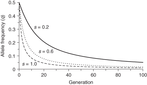
Equation (6.8) also shows the effect of the intensity of selection as measured by the selection coefficient s. For any given value of q, higher values of s will result in more allele frequency change, which means a faster approach to the final equilibrium value. This is intuitive—the greater the intensity of selection, the sooner it will occur. The effect of different values of s is shown in Figure 6.4. Higher values of s (which indicates lower fitness of the recessive homozygote) results in faster change over time. One of the curves in Figure 6.4 is particularly informative: the case of complete selection against the recessive homozygote. This case (s = 0) corresponds to a lethal recessive allele where any individual having two copies of the recessive allele will not survive and reproduce. An example in humans is Tay–Sachs disease, caused by a lethal recessive allele. Individuals that receive the lethal recessive allele from both parents are homozygous and usually die in their first few years of life. Since virtually none of the recessive homozygotes survive, does this mean that the lethal allele will be eliminated in a single generation? As seen in Figure 6.4, the answer is no, but this result might take a little bit of thought. If all of the recessive homozygotes die before reproducing, then how can any of the alleles continue? The answer, of course, is that heterozygotes carry one lethal allele and can pass it on to the next generation. Even when a recessive allele is lethal, it takes time to remove it from the population.

Figure 6.4 Selection against the recessive homozygote for different values of the selection coefficient. Initial allele frequencies are p = 0.5 and q = 0.5 in each case. Fitness values are wAA = 1, wAa = 1, and waa = 1 − s. Allele frequencies were derived using equation (6.7) for three different values of the selection coefficient: s = 0.2, s = 0.6, and s = 1.0.

6.3.2 Selection against Dominant Alleles

Now that we have seen the derivation of a general model of natural selection and worked through an example in depth, we can consider different forms of natural selection. For example, what happens if the situation discussed above is reversed and we have selection against a dominant allele? In this scenario, the fitness of both the dominant homozygote (AA) and the heterozygote (Aa) would be reduced relative to the recessive homozygote (aa). We start by writing the fitness values for each genotype to reflect these differences:

Mean fitness is derived by substituting these values into equation (6.1), giving

6.9

(see Appendix 6.8). This equation shows us that for any value of s, mean fitness will increase as the frequency of the recessive allele (q) increases (and, therefore, as the frequency of the dominant allele decreases).

Since we are interested in the frequency of the dominant allele, we use equation (6.2) to express the allele frequency p′ in the next generation, and substitute equation (6.9) for mean fitness, giving

6.10

The amount of change in the dominant allele per generation is now obtained from equation (6.4), giving

6.11

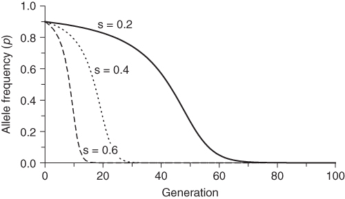
(see Appendix 6.8 for derivations). This equation shows us two important facts about selection against genotypes having the dominant allele: (1) Δp will always be negative (because of the negative sign in the numerator), and the frequency of p will always decrease over time, which makes sense as it is being selected against in this example; and (2) this decrease will continue until equilibrium, defined when Δp = 0. We see that this will occur when p = 0. Selection against the dominant allele will eventually remove the allele from the population. In this case, removal is complete as the dominant allele is expressed in the heterozygote, and therefore cannot be retained indefinitely in the population (even in a mathematical sense). As shown in Figure 6.5, higher values of s will remove the dominant allele more quickly.

Figure 6.5 Selection against dominant alleles. Initial allele frequencies are p = 0.9 for the dominant allele (A) and q = 0.1 for the recessive allele (a). Fitness values are wAA = 1 − s, wAa = 1 − s, and waa = 1. Allele frequencies were derived using equation (6.10) for three different values of the selection coefficient: s = 0.2, s = 0.4, and s = 0.6.

An interesting feature of selection against a dominant allele is that it is possible to remove the dominant allele in a single generation. This will happen when the dominant allele is lethal, such that anyone having either the AA or Aa genotype will be eliminated in the first generation, and only those with the recessive homozygote aa will survive. We can also see this effect mathematically by using complete selection (s = 1) in equation (6.10), which shows that if we start with allele frequency p, the frequency of the dominant allele in the next generation will be

This is the only way that selection can remove an allele in a single generation.

6.3.3 Selection with Codominant Alleles

The examples presented thus far have involved a dominant allele and a recessive allele. The next model considers that happens when the two alleles are codominant and there is selection against one of the alleles. Under codominance, the heterozygote Aa will show the effect of both alleles. One way to model selection in this type of situation is consider selection for the A allele and selection against the a allele. This is done by assigning the highest fitness to individuals with two A alleles (genotype AA), the lowest fitness to someone with no A alleles (genotype aa), and an intermediate fitness to those with one A allele (genotype Aa). The fitness values in this case are

Note that the fitness of the heterozygote is the average of the fitness values of the two homozygotes, thus meeting our criterion that the fitness of the heterozygote is intermediate:

Mean fitness is derived by substituting these values into equation (6.1), giving

6.12

(see Appendix 6.9). This equation shows us that for any value of s, mean fitness will increase as q decreases. Selection against the a allele will lead to its decline even under codominance.

The frequency of the a allele in the next generation is specifically derived by substituting the fitness values into equation (6.3), which gives

6.13

The amount of change in the a allele per generation is now obtained from equation (6.5), giving

6.14

(see Appendix 6.9). This equation has a negative sign in the numerator, which means that the frequency of the a allele decreases with each generation. This decrease will continue until Δq = 0, which will occur when q = 0. As with selection against the recessive homozygote, this is a mathematical limit.

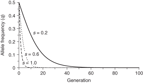
Figure 6.6 shows selection against the codominant allele a for three different values of the selection coefficient. As with selection against the recessive homozygote (Figure 6.4), the allele frequency decreases rapidly at first, approaching a value of zero. Note, however, that the rate of change of the examples shown in Figure 6.6 is faster (i.e., descent of the curves is steeper) than those shown in Figure 6.4 for the same selection coefficients. For example, under selection against the recessive homozygote for s = 0.2, the allele frequency drops from q = 0.5 to about q = 0.2 (Figure 6.4) after 20 generations, whereas the frequency drops to q = 0.1 after 20 generations of selection against the codominant allele (Figure 6.6). The reason for this is that the fitness of the heterozygote is lower for the case of selection against the codominant allele. Under selection against the recessive homozygote, no heterozygotes are selected against (because fitness = 1), whereas some heterozygotes are selected against under codominance (where fitness = 1 − s/2).

Figure 6.6 Selection against the codominant allele a for different values of the selection coefficient. Initial allele frequencies are p = 0.5 and q = 0.5 in each case. Fitness values are wAA = 1, wAa = 1 − (s/2), and waa = 1 − s. Allele frequencies were derived using equation (6.13) for three different values of the selection coefficient: s = 0.2, s = 0.6, and s = 1.0. Compare the rates of change here with the case of selection against the recessive homozygote shown in Figure 6.4.

Stay updated, free articles. Join our Telegram channel

Join