Key Terms
Accuracy
AMR
Bias
CLIA
Constant error
CRR
Descriptive statistics
Dispersion
Histograms
Levey-Jennings control chart
Limit of detection
Linear regression
Precision
Predictive values
Proficiency testing
Proportional error
Quality control
Random error
Reference interval
Reference method
SDI
Sensitivity
Shifts
Specificity
Systematic error
Trends
It is widely accepted that the majority of medical decisions are supported using laboratory data. It is therefore critical that results generated by the laboratory are accurate and provide the appropriate laboratory diagnostic information to assist the health care provider in treating patients. Determining and maintaining accuracy requires considerable effort and cost, entailing the use of a series of approaches depending on the complexity of the test. To begin, one must appreciate what quality is and how quality is measured and managed. To this end, it is vital to understand basic statistical concepts that enable the laboratorian to measure quality. Before implementing a new test, it is important to determine if the test is capable of performing acceptably by meeting or exceeding defined quality criteria; method evaluation is used to verify the acceptability of new methods prior to reporting patient results. Once a method has been implemented, it is essential that the laboratory ensures it remains valid over time; this is achieved by a process known as quality control (QC) and Quality Improvement/Assurance (see Chapter 4). This chapter describes basic statistical concepts and provides an overview of the procedures necessary to implement a new method and ensure its continued accuracy.
BASIC CONCEPTS
Each day, high-volume clinical laboratories generate thousands of results. This wealth of clinical laboratory data must be summarized and critically be reviewed to monitor test performance. The foundation for monitoring performance (known as QC) is descriptive statistics.
Descriptive Statistics: Measures of Center, Spread, and Shape
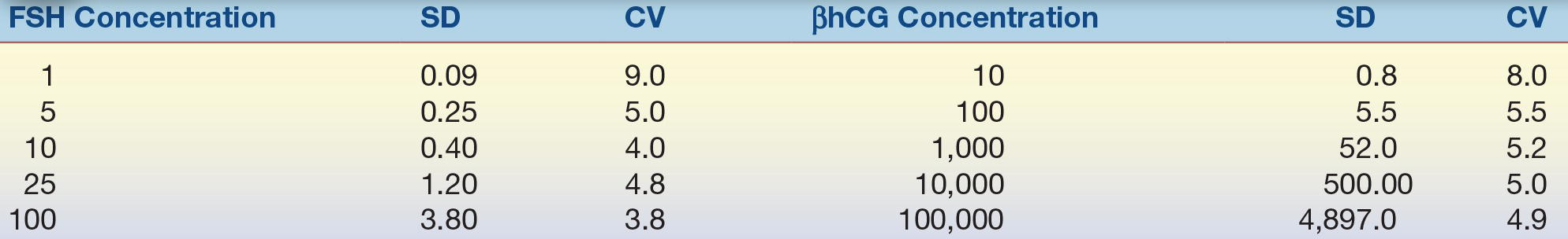
When examined closely, a collection of seemingly similar things always has at least slight differences for any given characteristic (e.g., smoothness, size, color, weight, volume, and potency). Similarly, laboratory data will have at least slight measurement differences. For example, if glucose on a given specimen is measured 100 times in a row, there would be a range of values obtained. Such differences in laboratory values can be a result of a variety of sources. Although measurements will differ, their values form patterns that can be visualized and analyzed collectively. Laboratorians view and describe these patterns using graphical representations and descriptive statistics (Fig. 3.1).
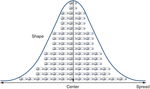
FIGURE 3.1 Basic measures of data include the center, spread, and shape.
When comparing and analyzing collections or sets of laboratory data, patterns can be described by their center, spread, and shape. Although comparing the center of data is most common, comparing the spread can be even more powerful. Assessment of data dispersion, or spread, allows laboratorians to assess the predictability (and the lack of) in a laboratory test or measurement.
Measures of Center
The three most commonly used descriptions of the center of a data set (Fig. 3.2) are the mean, the median, and the mode. The mean is most commonly used and often called the average. The median is the “middle” point and is often used with skewed data so its calculation is not significantly affected by outliers. The mode is rarely used as a measure of the data’s center but is more often used to describe data that seem to have two centers (i.e., bimodal). The mean is calculated by summing the observations and dividing by the number of the critically evaluated observations (Box 3.1).
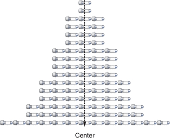
FIGURE 3.2 The center can be defined by the mean (x-bar character), median, or mode.
 BOX 3.1 Sources of Analytic Variability
Mean Equation:
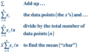 (Eq. 3-1)
 The summation sign, Σ, is an abbreviation for (x1 + x2 + x3 + ··· + xn) and is used in many statistical formulas. Often, the mean of a specific data set is called  or “x bar.”
The median is the middle of the data after the data have been rank ordered. It is the value that divides the data in half. To determine the median, values are rank ordered from least to greatest and the middle value is selected. For example, given a sample of 5, 4, 6, 5, 3, 7, 5, the rank order of the points is 3, 4, 5, 5, 5, 6, 7. Because there are an odd number of values in the sample, the middle value (median) is 5; the value 5 divides the data in half. Given another sample with an even number of values 5, 4, 6, 8, 9, 7, the rank order of the points is 4, 5, 6, 7, 8, 9. The two “middle” values are 6 and 7. Adding them yields 13 (6 + 7 = 13); division by 2 provides the median (13/2 = 6.5). The median value of 6.5 divides the data in half.
The mode is the most frequently occurring value in a data set. Although it is seldom used to describe data, it is referred to when in reference to the shape of data, a bimodal distribution, for example. In the sample 3, 4, 5, 5, 5, 6, 7, the value that occurs most often is 5. The mode of this set is then 5. The data set 3, 4, 5, 5, 5, 6, 7, 8, 9, 9, 9 has two modes, 5 and 9.
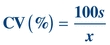
After describing the center of the data set, it is very useful to indicate how the data are distributed (spread). The spread represents the relationship of all the data points to the mean (Fig. 3.3). There are four commonly used descriptions of spread: (1) range, (2) standard deviation (SD), (3) coefficient of variation (CV), and (4) standard deviation index (SDI). The easiest measure of spread to understand is the range. The range is simply the largest value in the data minus the smallest value, which represents the extremes of data one might encounter. Standard deviation (also called “s,” SD, or σ) is the most frequently used measure of variation. Although calculating SD can seem somewhat intimidating, the concept is straightforward; in fact, all of the descriptive statistics and even the inferential statistics have a combination of mathematical operations that are by themselves no more complex than a square root. The SD and, more specifically, the variance represent the “average” distance from the center of the data (the mean) and every value in the data set. The CV allows a laboratorian to compare SDs with different units and reflects the SDs in percentages. The SDI is a calculation to show the number of SDs a value is from the target mean. Similar to CV, it is a way to reflect ranges in a relative manner regardless of how low or high the values are.
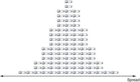
FIGURE 3.3 Spread is defined by the standard deviation and coefficient of variation.
Range is one description of the spread of data. It is simply the difference between the highest and lowest data points: range = high − low. For the sample 5, 4, 6, 5, 3, 7, 5, the range is 7 − 3 = 4. The range is often a good measure of dispersion for small samples of data. It does have a serious drawback; the range is susceptible to extreme values or outliers (i.e., wrong quality control material or wrong data entry).
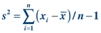
To calculate the SD of a data set, it is easiest to first determine the variance (s2). Variance is similar to the mean in that it is an average. Variance is the average of the squared distances of all values from the mean:
 (Eq. 3-2)
 As a measure of dispersion, variance represents the difference between each value and the average of the data. Given the values 5, 4, 6, 5, 3, 7, 5, variance can be calculated as shown below:
 (Eq. 3-3)
 To calculate the SD (or “s”), simply take the square root of the variance:
 (Eq. 3-4)
 Although it is important to understand how these measures are calculated, most analyzer/instruments, laboratory information systems, and laboratory statistical software packages determine these automatically. SD describes the distribution of all data points around the mean.
Another way of expressing SD is in terms of the CV. The CV is calculated by dividing the SD by the mean and multiplying by 100 to express it as a percentage:
 (Eq. 3-5)
 The CV simplifies comparison of SDs of test results expressed in different units and concentrations. As shown in Table 3.1, analytes measured at different concentrations can have a drastically different SD but a comparable CV. The CV is used extensively to summarize QC data. The CV of highly precise analyzers can be lower than 1%. For values at the low end of the analytical measurement, the acceptable CV can range as high as 50% as allowed by CLIA.
TABLE 3.1 Comparison of SD and CV for Two Different Analytes
SD, standard deviation; CV, coefficient of variation; FSH, follicle-stimulating hormone; βhCG, β-human chorionic gonadotropin.
Another way of expressing SD is in terms of the SDI, where the SDI is calculated by dividing the difference of the (measured laboratory value or mean − target or group mean)/assigned or group SD. The SDI can be a negative or positive value.
 (Eq. 3-6)
 Measures of Shape
Although there are hundreds of different “shapes”— distributions—that data sets can exhibit, the most commonly discussed is the Gaussian distribution (also called normal distribution; Fig. 3.4). The Gaussian distribution describes many continuous laboratory variables and shares several unique characteristics: the mean, median, and mode are identical; the distribution is symmetric—meaning half the values fall to the left of the mean and the other half fall to the right with the peak of the curve representing the average of the data. This symmetrical shape is often called a “bell curve.”
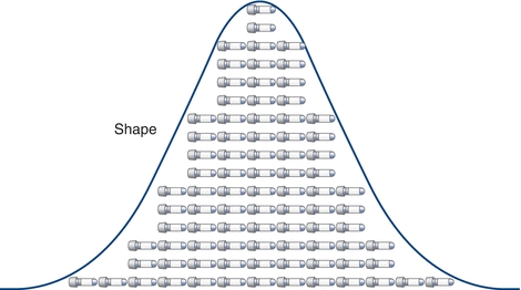
FIGURE 3.4 Shape is defined by how the distribution of data relates the center. This is an example of data that have “normal” or Gaussian distribution.
The total area under the Gaussian curve is 1.0, or 100%. Much of the area—68.3%—under the “normal” curve is between ±1 SD (μ ± 1σ) (Fig. 3.5A). Most of the area—95.4%—under the “normal” curve is between ±2 SDs (μ ± 2σ; Fig. 3.5B). And almost all of the area—99.7%—under the “normal” curve is between ±3 SDs (μ ± 3σ) (Fig. 3.5C). (Note that μ represents the average of the total population, whereas the mean of a specific data set is  or “x bar.”)
FIGURE 3.5 A normal distribution contains (A) ≈68% of the results within ±1 SD (1s or 1σ), (B) 95% of the results within ±2s (2σ), and (C) ≈99% of the results within ±3σ.
The “68–95–99 Rule” summarizes the above relationships between the area under a Gaussian distribution and the SD. In other words, given any Gaussian distributed data, ≈68% of the data fall between ±1 SD from the mean; ≈95% of the data fall between ±2 SDs from the mean; and ≈99% fall between ±3 SDs from the mean. Likewise, if you selected a value in a data set that is Gaussian distributed, there is a 0.68 chance of it lying between ±1 SD from the mean; there is a 0.95 likelihood of it lying between ±2 SDs; and there is a 0.99 probability of it lying between ±3 SDs. (Note: the terms “chance,” “likelihood,” and “probability” are synonymous in this example.)
As will be discussed in the reference interval section, most patient data are not normally distributed. These data may be skewed or exhibit multiple centers (bimodal, trimodal, etc.) as shown in Figure 3.6. Plotting data in histograms as shown in the figure is a useful and an easy way to visualize distribution. However, there are also mathematical analyses (e.g., normality tests) that can confirm if data fit a given distribution. The importance of recognizing whether data are or are not normally distributed is related to the way it can be statistically analyzed.
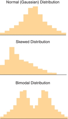
FIGURE 3.6 Examples of normal (Gaussian), skewed, and bimodal distributions. The type of statistical analysis that is performed to analyze the data depends on the distribution (shape).
Descriptive Statistics of Groups of Paired Observations
While the use of basic descriptive statistics is satisfactory for examining a single method, laboratorians frequently need to compare two different methods. This is most commonly encountered in comparison of methods (COM) experiments. A COM experiment involves measuring patient specimens by both an existing (reference) method and a new (test) method (described in the Reference Interval and Method Evaluation sections later). The data obtained from these comparisons consist of two measurements for each patient specimen. It is easiest to visualize and summarize the paired-method comparison data graphically (Fig. 3.7). By convention, the values obtained by the reference method are plotted on the x-axis, and the values obtained by the test method are plotted on the y-axis.
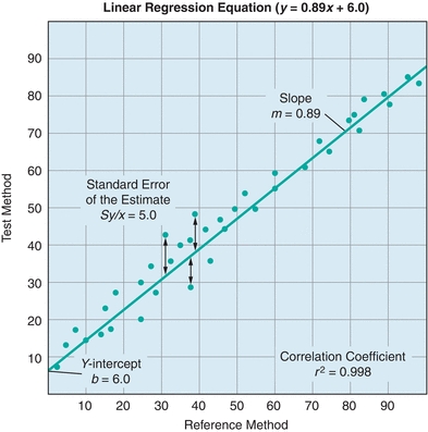
FIGURE 3.7 A generic example of a linear regression. A linear regression compares two tests and yields important information about systematic and random error. Systematic error is indicated by changes in the y-intercept (constant error) and the slope (proportional error). Random error is indicated by the standard error of the estimate (Sy/x); Sy/x basically represents the distance of each point from the regression line. The correlation coefficient indicates the strength of the relationship between the tests.
In Figure 3.7, the agreement between the two methods is estimated from the straight line that best fits the points. Whereas visual estimation may be used to draw the line, a statistical technique known as linear regression analysis provides objective an objective measure of the line of best fit for the data. Three factors are generated in a linear regression—the slope, the y-intercept, and the correlation coefficient (r). In Figure 3.7, there is a linear relationship between the two methods over the entire range of values. The linear regression is defined by the equation y = mx + b. The slope of the line is described by m, and the value of the y-intercept (b) is determined by plugging x = 0 into the equation and solving for y. The correlation coefficient (r) is a measure of the strength of the relationship between the two methods. The correlation coefficient can have values from −1 to 1, with the sign indicating the direction of relationship between the two variables. A positive r indicates that both variables increase and decrease together, whereas a negative r indicates that as one variable increases, the other decreases. An r value of 0 indicates no relationship, whereas r = 1.0 indicates a perfect relationship. Although many equate high positive values of r (0.95 or higher) with excellent agreement between the test and comparative methods, most clinical chemistry comparisons should have correlation coefficients greater than 0.98. When r is less than 0.99, the regression formula can underestimate the slope and overestimate the y-intercept. The absolute value of the correlation coefficient can be increased by widening the concentration range of samples being compared. However, if the correlation coefficient remains less than 0.99, then alternate regression statistics or modified COM value sets should be used to derive more realistic estimates of the regression, slope, and y-intercept.1,2 Visual inspection of data is essential prior to drawing conclusions from the summary statistics as demonstrated by the famous Anscombe quartet (Fig. 3.8). In this data set, the slope, y-intercept, and correlation coefficients are all identical, yet visual inspection reveals that the underlying data are completely different.
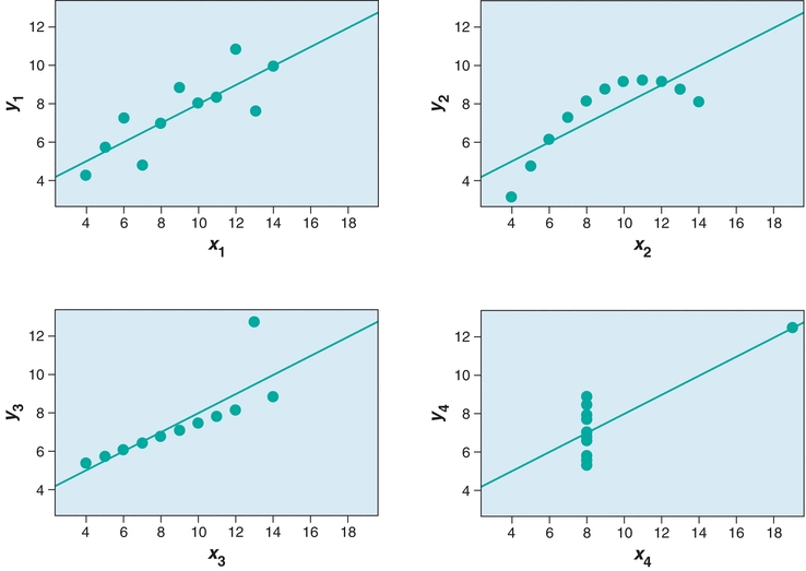
FIGURE 3.8 Anscombe’s quartet demonstrates the need to visually inspect data. In each panel, y = 0.5 x + 3, r2 = 0.816, Sy/x = 4.1.
An alternate approach to visualizing paired data is the difference plot, which is also known as the Bland-Altman plot (Fig. 3.9). A difference plot indicates either the percent or absolute bias (difference) between the reference and test method values over the average range of values. This approach permits simple comparison of the differences to previously established maximum limits. As is evident in Figure 3.9, it is easier to visualize any concentration-dependent differences than by linear regression analysis. In this example, the percent difference is clearly greatest at lower concentrations, which may not be obvious from a regression plot.
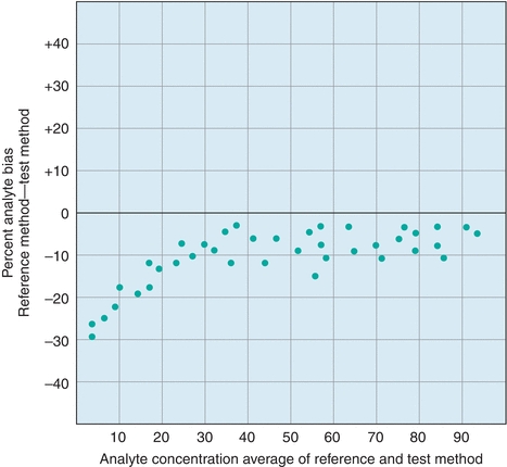
FIGURE 3.9 An example of a difference (Bland-Altman) plot. Difference plots are a useful tool to visualize concentration-dependent error.
The difference between test and reference method results is called error. There are two kinds of error measured in COM experiments: random and systematic. Random error is present in all measurements and can be either positive or negative, typically a combination of both positive and negative errors on both sides of the assigned target value. Random error can be a result of many factors including instrument, operator, reagent, and environmental variation. Random error is calculated as the SD of the points about the regression line (Sy/x). Sy/x essentially refers to average distance of the data from the regression line (Fig. 3.7). The higher the Sy/x, the wider is the scatter and the higher is the amount of random error. In Figure 3.7, the Sy/x is 5.0. If the points were perfectly in line with the linear regression, the Sy/x would equal 0.0, indicating there would not be any random error. Sy/x is also known as the standard error of the estimate SE (Box 3.2).
 BOX 3.2 Types of Error in Laboratory Testing: a Preview of Things to Come

Systematic error influences observations consistently in one direction (higher or lower). The measures of slope and y-intercept provide estimates of the systematic error. Systematic error can be further broken down into constant error and proportional error. Constant systematic error exists when there is a continual difference between the test method and the comparative method values, regardless of the concentration. In Figure 3.7, there is a constant difference of 6.0 between the test method values and the comparative method values. This constant difference, reflected in the y-intercept, is called constant systematic error. Proportional error exists when the differences between the test method and the comparative method values are proportional to the analyte concentration. Proportional error is present when the slope is 1. In the example, the slope of 0.89 represents the proportional error, where samples will be underestimated in a concentration-dependent fashion by the test method compared with the reference method; the error is proportional, because it will increase with the analyte concentration.
Inferential Statistics
The next level of complexity beyond paired descriptive statistics is inferential statistics. Inferential statistics are used to draw conclusions (inferences) regarding the means or SDs of two sets of data. Inferential statistical analyses are most commonly encountered in research studies, but can also be used in COM studies.
An important consideration for inferential statistics is the distribution of the data (shape). The distribution of the data determines what kind of inferential statistics can be used to analyze the data. Normally distributed (Gaussian) data are typically analyzed using what are known as “parametric” tests, which include a Student’s t-test or analysis of variance (ANOVA). Data that are not normally distributed require a “nonparametric” analysis. Nonparametric tests are encountered in reference interval studies, where population data are often skewed. For reference interval studies, nonparametric methods typically rely on ranking or ordering the values in order to determine upper and lower percentiles. While many software packages are capable of performing either parametric or nonparametric analyses, it is important for the user to understand that the type of data (shape) dictates which statistical test is appropriate for the analysis. An inappropriate analysis of sound data can yield the wrong conclusion and lead to erroneous provider decisions and patient care/impact consequences.
METHOD EVALUATION
The value of clinical laboratory service is based on its ability to provide reliable, accurate test results and optimal test information for patient management. At the heart of providing these services is the performance of a testing method. To maximize the usefulness of a test, laboratorians undergo a process in which a method is selected and evaluated for its usefulness to those who will be using the test. This process is carefully undertaken to produce results within medically acceptable error limits to help providers maximally manage/treat their patients.
Currently, clinical laboratories more often select and evaluate methods that were commercially developed instead of developing their own. Most commercially developed tests have U.S. Food and Drug Administration (FDA) approval, only requiring a laboratory to provide a limited but regulatory mandated evaluation of a method to verify the manufacturer’s performance claims and to see how well the method works specifically in the laboratory and patient population served.
Regulatory Aspects of Method Evaluation (Alphabet Soup)
The Centers for Medicare and Medicaid Services (CMS) and the Federal Drug Agency (FDA) are the primary government agencies that influence laboratory testing methods in the United States. The FDA regulates laboratory instruments and reagents, and the CMS regulates the Clinical Laboratory Improvement Amendments (CLIA).3 Most large laboratories in the United States are accredited by the College of American Pathologists (CAP) and The Joint Commission (TJC; formerly the Joint Commission on Accreditation of Healthcare Organizations [JCAHO]), which impacts how method evaluations need to be performed. Professional organizations such as the National Academy of Clinical Biochemistry (NACB) and the American Association for Clinical Chemistry (AACC) also contribute important guidelines and method evaluations that influence how method evaluations are performed. Future trends are seeing additional regulatory services being used by both larger laboratories and smaller laboratories (i.e., Physician clinics and public health departments), Commission of Office Laboratory Accreditation (COLA) is an example of additional regulatory services available to clinical laboratories regardless of their size, test menu, and test volume. Regardless of which regulatory agency is used the acceptable and mandatory standards of compliance guidelines are set by CLIA, FDA, and TJC.
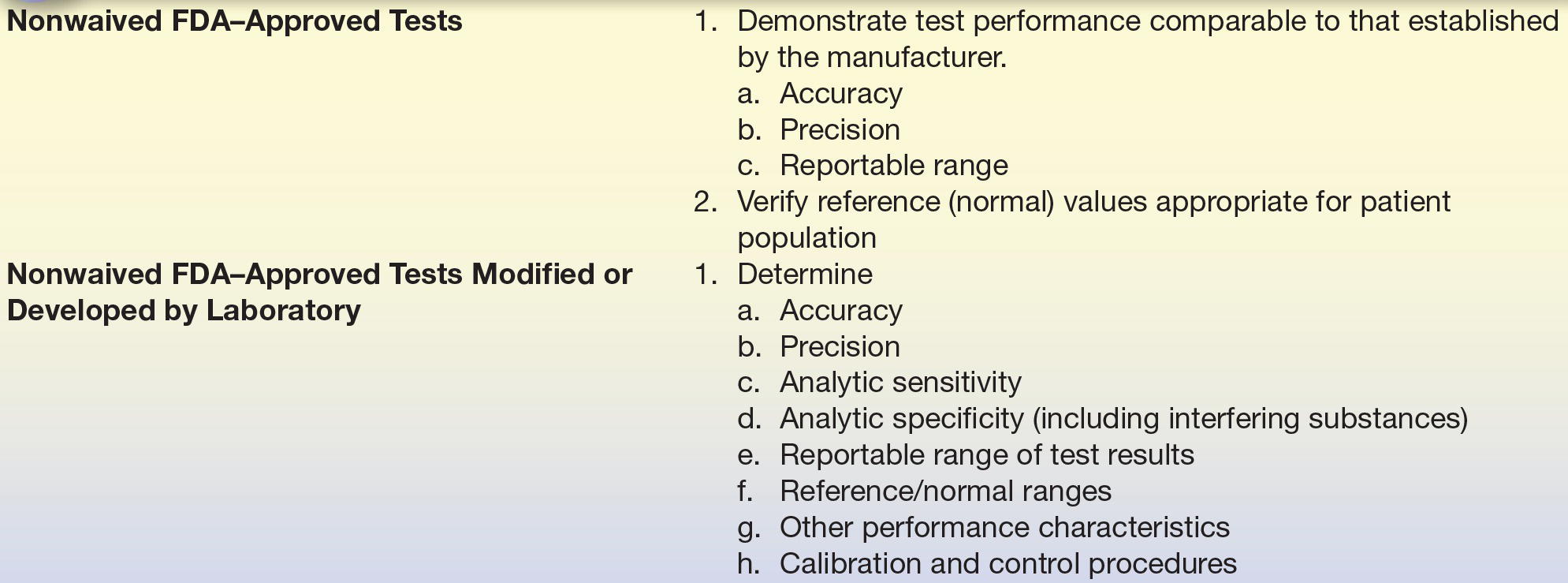
The FDA “Office of In Vitro Diagnostic Device Evaluation and Safety” (OIVD) regulates diagnostic tests. Tests are categorized into one of three groups: (1) waived, (2) moderate complexity, and (3) high complexity. Waived tests are cleared by the FDA to be so simple that they are most likely accurate and most importantly would pose negligible risk of harm to the patient if not performed correctly. A few examples of waived testing include dipstick tests, qualitative pregnancy testing, rapid strep, rapid HIV, rapid HCV, and glucose monitors. For waived testing, personnel requirements are not as stringent as moderately complex testing or high-complexity testing, but there are still training, competency, and quality control mandatory requirements. Most automated methods are rated as moderate complexity, while manual methods and methods requiring more interpretation are rated as high complexity. The patient management/treatment impact is also a factor in determining whether a test is waived, moderate complexity or high complexity. The CLIA final rule requires that waived tests simply follow the manufacturer’s instructions. Both moderate- and high-complexity tests require in-laboratory validation. However, FDA-approved nonwaived tests may undergo a more basic validation process (Table 3.2), whereas a more extensive validation is required for tests developed by laboratories (Table 3.2). While the major requirements for testing validation are driven by the CLIA, TJC and CAP essentially require the same types of experiments to be performed, with a few additions. It is these rules that guide the way tests in the clinical chemistry laboratory are selected and validated.
TABLE 3.2 General CLIA Regulations of Method Validation
From Clinical Laboratory Improvement Amendments of 1988; final rule. Fed Regist. 7164 [42 CFR 493 1253]: Department of Health and Human Services, Centers for Medicare and Medicaid Services; 1992.
DEFINITIONS BOX
Method Selection
Evaluating a method is a labor-intensive costly process—so why select a new method? There are many reasons, including enhanced provider utilization in effectively treating/managing patients, reducing costs, staffing needs, improving the overall quality of results, increasing provider satisfaction, and improving overall efficiency. Selecting a test method starts with the collection of technical information about a particular test from colleagues, scientific presentations, the scientific literature, and manufacturer claims. Practical considerations should also be addressed at this point, such as the type and volume of specimen to be tested, the required throughput and turnaround time, your testing needs, testing volumes, cost, break-even financial analysis, calibration, Quality Control Plan, space needs, disposal needs, personnel requirements, safety considerations, alternative strategies to supply testing (i.e., referral testing laboratories), etc. Most importantly, the test should be able to meet the clinical task by having specific analytic performance standards that will accurately assist in the management and ultimately the treatment of patients. Specific information that should be discovered about a test you might bring into the laboratory includes analytic sensitivity, analytic specificity, linear range, interfering substances, estimates of precision and accuracy, and test-specific regulatory requirements. The process of method selection is the beginning of a process to bring in a new test for routine use (Fig. 3.10).
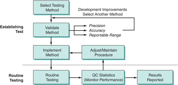
FIGURE 3.10 A flowchart on the process of method selection, evaluation, and monitoring. (Adapted from Westgard JO, Quam E, Barry T. Basic QC Practices: Training in Statistical Quality Control for Healthcare Laboratories. Madison, WI: Westgard Quality Corp.; 1998.)
Method Evaluation
A short, initial evaluation should be carried out before the complete method evaluation. This preliminary evaluation should include the analysis of a series of standards to verify the linear range and the replicate analysis (at least eight measurements) of two controls to obtain estimates of short-term precision. If any results fall short of the specifications published in the method’s product information sheet (package insert), the method’s manufacturer should be consulted. Without a successful initial evaluation, including precision and linear range minimal studies, there is no opportunity to proceed with the method evaluation until the initial issues have been resolved. Also, without improvement in the method, more extensive evaluations are pointless.4
First Things First: Determine Imprecision and Inaccuracy
The first determinations (estimates) to be made in a method evaluation are the precision and accuracy, which should be compared with the maximum allowable error budgets based on medical criteria and regulatory guidelines. If the precision or accuracy exceeds the maximum allowable error budgets, it is unacceptable and must be modified and reevaluated or rejected. Precision is the dispersion of repeated measurements around a mean (true level), as shown in Figure 3.11A with the mean represented as the bull’s-eye. Random analytic error is the cause of lack of precision or the imprecision in a test. Precision is estimated from studies in which multiple aliquots of the same specimen (with a constant concentration) are analyzed repetitively.
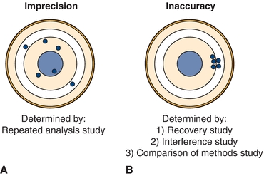
FIGURE 3.11 Graphic representation of (A) imprecision and (B) inaccuracy on a dartboard configuration with bull’s-eye in the center.
Accuracy, or the difference between a measured value and its actual value, is due to the presence of a systematic error, as represented in Figure 3.11B. Systematic error can be due to constant or proportional error and is estimated from three types of study: (1) recovery, (2) interference, and (3) a COM study.
DEFINITIONS BOX
DEFINITIONS BOX
Measurement of Imprecision
Method evaluation begins with a precision study. This estimates the random error associated with the test method and detects any problems affecting its reproducibility. It is recommended that this study be performed over a 10- to 20-day period, incorporating one or two analytic runs (runs with patient samples or QC materials) per day, preferred is an AM run and a PM run.5,6 A common precision study is a 2 × 2 × 10 study, where two controls are run twice a day (AM and PM) for 10 days. The rationale for performing the evaluation of precision over many days is logical. Running multiple samples on the same day does a good job of estimating precision within a single day (simple precision) but underestimates long-term changes and testing variables that occur over time. By running multiple samples on different days, a better estimation of the random error over time is given. It is important that more than one concentration be tested in these studies, with materials ideally spanning the clinically appropriate and analytical measurement range of concentrations. For glucose, this might include samples in the hyperglycemic range (150 mg/dL) and the hypoglycemic range (50 mg/dL). After these data are collected, the mean, SD, CV, and SDI are calculated. An example of a precision study from our laboratory is shown in Figure 3.12.
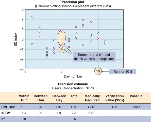
FIGURE 3.12 An example of a precision study for vitamin B12. The data represent analysis of a control sample run in duplicate twice a day (red and black circles) for 10 days (x-axis). Data are presented as standard deviation index (SDI). SDI refers to the difference between the measured value and the mean expressed as a number of SDs. An imprecision study is designed to detect random error.
The random error or imprecision associated with the test procedure is indicated by the SD and the CV. The within-run imprecision is indicated by the SD of the controls analyzed within one run. The total imprecision may be obtained from the SD of control data with one or two data points accumulated per day. The total imprecision is the most accurate assessment of performance that would affect the values a provider might see and reflects differences in operators, pipettes, and variations in environmental changes such as temperature, reagent stability, etc. In practice, however, within-run imprecision is used more commonly than total imprecision. An inferential statistical technique, ANOVA, is then used to analyze the available precision data to provide estimates of the within-run, between-run, and total imprecision.7
Acceptable Performance Criteria: Precision Studies
During an evaluation of vitamin B12 in the laboratory, a precision study was performed for a new test method (Fig. 3.12). Several concentrations of vitamin B12 were run twice daily (in duplicate) for 10 days, as shown in Figure 3.12 (for simplicity, only one concentration is shown). The data are represented in the precision plot in Figure 3.12 (≈76 pg/mL). The amount of variability between runs is represented by different colors, over 10 days (x-axis). The CV was then calculated for within-run, between-run, and between-days. The total SD, estimated at 2.3, is then compared with medical decision levels or medically required standards based on the analyte (Table 3.3). The acceptability of analytic error is based on how the test is to be used to make clinical interpretations.8,9 In this case, the medically required SD limit is 4.8, based on mandated CLIA error budgets. The determination of whether long-term precision is adequate is based on the total imprecision being less than one-third of the total allowable error (total imprecision, in this case, 1.6; selection of one-third total allowable error for imprecision is based on Westgard10). In the case that the value is greater than the total allowable error (1.79 in our example), the test can pass as long as the difference between one-third total allowable error and the determined allowable error is not statistically significant. In our case, the 1.79 was not statistically different from 1.6 (1/3 × 4.8), and the test passed our imprecision studies (Fig. 3.12). The one-third of total error is a run of thumb; some laboratories may choose one-fourth of the total error for analytes that are very precise and accurate. It is not recommended to use all of the allowable error for imprecision (random error) as it leaves no room for systematic error (bias or inaccuracy).
TABLE 3.3 Performance Standards for Common Clinical Chemistry Analytes as Defined by the CLIA
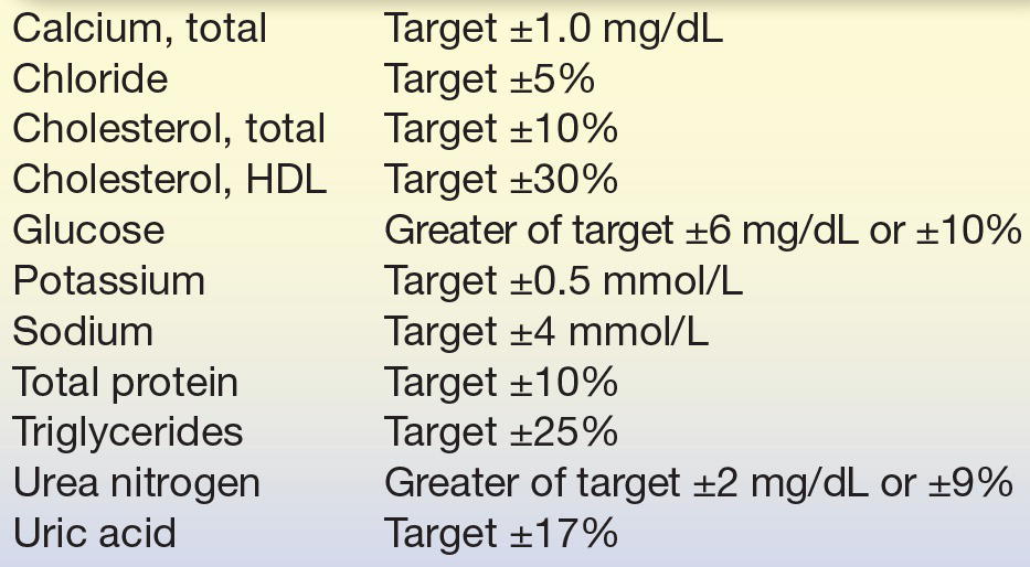
Reprinted from Centers for Disease Control and Prevention (CDC), Centers for Medicare and Medicaid Services (CMS), Health and Human Services. Medicare, Medicaid, and CLIA programs; laboratory requirements relating to quality systems and certain personnel qualifications. Final rule. Fed Regist. 2003;68:3639–3714, with permission.
DEFINITIONS BOX
Estimation of Inaccuracy
Once method imprecision is estimated and deemed acceptable, the determination of accuracy can begin.6 Accuracy is estimated using three different types of studies: (1) recovery, (2) interference, and (3) patient sample comparison.
Recovery Studies
Recovery studies will show whether a method is able to accurately measure an analyte. In a recovery experiment, a small aliquot of concentrated analyte is added (spiked) into a patient sample (matrix) and then measured by the method being evaluated. The amount recovered is the difference between the spiked sample and the patient sample (unmodified). The purpose of this type of study is to determine how much of the analyte can be detected (recovered) in the presence of all the other compounds in the matrix. The original patient samples (matrix) should not be diluted more than 10% so that the physiological (biological and protein components) matrix solution is minimally affected. An actual example of a recovery study for total calcium is illustrated in Figure 3.13; the results are expressed as percentage recovered. The performance standard for calcium, defined by CLIA, is the target value ±1.0 mg/dL (see Table 3.3). Recovery of calcium in this example exceeds this standard at the two calcium levels tested and therefore acceptable (Fig. 3.13).
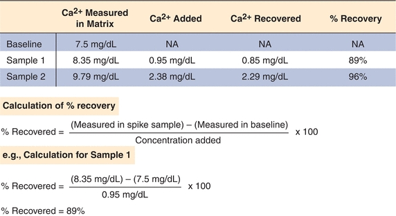
FIGURE 3.13 An example of a sample recovery study for total calcium. A sample is spiked with known amounts of calcium in a standard matrix, and recovery is determined as shown. Recovery studies are designed to detect proportional error in an assay.
Interference Studies
Interference studies are designed to determine if specific compounds affect the accuracy of laboratory tests. Common interferences encountered in the laboratory include hemolysis (broken red blood cells and their contents), icterus (high bilirubin), and turbidity (particulate matter or lipids), which can affect the measurement of many analytes. Interferents often affect tests by absorbing or scattering light, but they can also react with the reagents or affect reaction rates used to measure a given analyte.
Interference experiments are typically performed by adding the potential interferent to patient samples.11 If an effect is observed, the concentration of the interferent is lowered sequentially to determine the concentration at which test results are not clinically affected (or minimally affected). It is common practice to flag results with unacceptably high levels of an interferent. Results may be reported with cautionary comments or not reported at all. An example of an interference study performed in one laboratory is shown in Figure 3.14. When designing a method validation study, potential interferents should be selected from literature reviews and specific references. Other excellent resources include Young12 and Siest and Galteau.13 Common interferences, such as hemolysis, lipemia, bilirubin, anticoagulant, and preservatives, are tested by the manufacturer. Glick and Ryder14,15 published “interferographs” for clinical chemistry instruments, which relate analyte concentration measure to interferent concentration. They have also demonstrated that considerable expense can be saved by the acquisition of instruments that minimize hemoglobin, triglyceride, and bilirubin interference.16 It is good laboratory practice and a regulatory requirement to consider interferences as part of any method validation. In the clinical laboratory, interference studies “in vitro” are often difficult, and standardized experiments are often suspect as to reflecting the actual actions “in vivo.” Proper instrumentation and critical literature reviews are often the best options for determining interference acceptability guidelines.
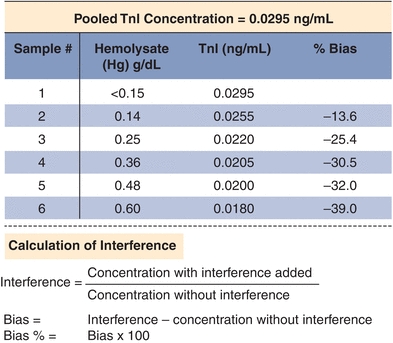
FIGURE 3.14 An example of an interference study for troponin I (TnI). Increasing amounts of hemolysate (lysed red blood cells, a common interference) were added to a sample with elevated TnI of 0.295 ng/mL. Bias is calculated based on the difference between the baseline and hemolyzed samples. The data are corrected for the dilution with hemolysate.
COM Studies
A method comparison experiment examines patient samples by the method being evaluated (test method) with a reference method. It is used primarily to estimate systematic error in actual patient samples, and it may offer the type of systematic error (proportional vs. constant). Ideally, the test method is compared with a standardized reference method (gold standard), a method with acceptable accuracy in comparison with its imprecision. Many times, reference methods are laborious and time consuming, as is the case with the ultracentrifugation methods of determining cholesterol. Because most laboratories are understaffed or do not have the technical expertise required to perform reference methods, most test methods are compared with those routinely used. These routine tests have their own particular inaccuracies, so it is important to determine what inaccuracies they might have that are documented in the literature. If the new test method is to replace the routine method, differences between the two should be well characterized. Also extensive documented communications with all providers and staff must be performed before implementation.
To compare a test method with a comparative method, it is recommended by Westgard et al.6 and CLIA17 that 40 to 100 specimens be run by each method on the same day over 8 to 20 days (preferably within 4 hours), with specimens spanning the clinical range and representing a diversity of pathologic conditions. Samples should cover the full analytical measurement range, and it is recommended that 25% be lower than the reference range, 50% should be in the reference range, and 25% should be higher than the reference range. Additional samples at the medical decision points should be a priority during the COM. As an extra measure of QC, specimens should be analyzed in duplicate. Otherwise, experimental results must be critically reviewed by the laboratory director and evaluation staff comparing test and comparative method results immediately after analysis. Samples with large differences should be repeated to rule out technical errors as the source of variation. Daily analysis of two to five patient specimens should be followed for at least 8 days if 40 specimens are compared and for 20 days if 100 specimens are compared in replication studies.17
A plot of the test method data (y-axis) versus the comparative method (x-axis) helps to visualize the data generated in a COM test (Fig. 3.15A).18 As described earlier, if the two methods correlate perfectly, the data pairs plotted as concentration values from the reference method (x) versus the evaluation method (y) will produce a straight line (y = mx + b), with a slope of 1.0, a y-intercept of 0, and a correlation coefficient (r) of 1. Data should be plotted daily and inspected for outliers so that original samples can be reanalyzed as needed. While linearity can be confirmed visually in most cases, it may be necessary to evaluate linearity more quantitatively.19
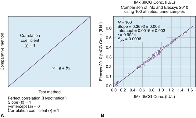
FIGURE 3.15 A comparison of methods experiment. (A) A model of a perfect method comparison. (B) An actual method comparison of beta-human chorionic gonadotropin (βhCG) between the Elecsys 2010 (Roche, Nutley, NJ) and the IMx (Abbott Laboratories, Abbott Park, IL). (Adapted from Shahzad K, Kim DH, Kang MJ. Analytic evaluation of the beta-human chorionic gonadotropin assay on the Abbott IMx and Elecsys2010 for its use in doping control. Clin Biochem. 2007;40:1259–1265.)
DEFINITIONS BOX
Statistical Analysis of COM Studies
While a visual inspection of method comparisons is essential, statistical analysis can be used to make objective decisions about the performance of a method. The first and most fundamental statistical analysis for COM studies is the linear regression. Linear regression analysis yields the slope (b), the y-intercept (a), the SD of the points about the regression line (Sy/x), and the correlation coefficient (r); regression also yields the coefficient of determination (r2) (see DEFINITIONS BOX). An example of these calculations can be found in Figure 3.15, where a comparison of β-human chorionic gonadotropin (βhCG) concentrations on an existing immunoassay system (Reference Method) and to a new system (Test Method). Statistics are calculated to determine the types and amounts of error that a method has, which is the basis for deciding if the test is still valid to make clinical decisions. Several types of errors can be seen looking at a plot of test method versus comparative method (Fig. 3.16). When random errors occur (Fig. 3.16A), points are randomly distributed around the regression line. Increases in the Sy/x statistic reflect random error. Constant error (Fig. 3.16B) is seen visually as a shift in the y-intercept; a t-test can be used to determine if two sets of data are significantly different from each other. Proportional error (Fig. 3.16C) is reflected in alterations in line slope and can also be analyzed with a t-test (see Fig. 3.1).
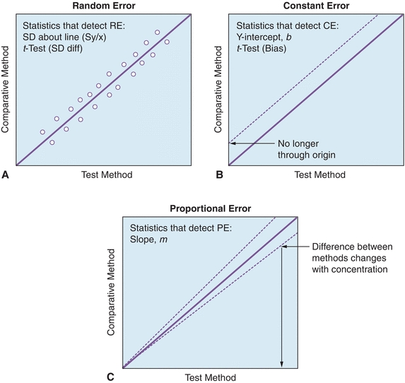
FIGURE 3.16 Examples of (A) random, (B) constant, and (C) proportional error using linear regression analysis. (Adapted from Westgard JO. Basic Method Evaluation. 2nd ed. Madison, WI: Westgard Quality Corp.; 2003.)
Stay updated, free articles. Join our Telegram channel

Full access? Get Clinical Tree


