Measures of Association for Ranked Data

The problem we now face is hopefully a familiar one: establishing a correlation between two sets of data. If we didn’t know any differently, we might proceed with a Pearson correlation. However, on reflection, the data obviously are not at all normal, on two counts.

First, the rankings of Amaze proficiency. Only one person is ranked 1, only one ranked 2, and so on, so that data have a rectangular distribution. Duration of labor might be better because it is measured in hours and minutes, except for one tiny detail. We have all heard tales of women who delivered in the taxi¹ 47 seconds after they went into labor. Conversely, middle-aged women seem to take perverse delight in regaling expectant first-time mothers with stories of Aunt Maude, who was in labor for 17 days and nights and then delivered triplets, unbeknownst to all, including the doctor. If there ever was a skewed distribution, duration of labor is likely it, and this is exactly the situation for which nonparametric statistical methods were invented. So it makes sense to begin by converting the raw data on duration to a ranking as well. An example of how the data might look after the exercise of ranking for 15 happy (hah!) moms is shown in Table 24–1.

We will now spend the next few pages delighting you with a few ways to approach the business of generating measures of association with these ranked data. But before we do, just to keep a perspective on the whole thing, we have proceeded to calculate a Pearson’s correlation on these data as an anchor point for what follows. It equals .89; keep that in mind.²

SPEARMAN’S RHO

The most common, most ancient, and most straightforward approach to measuring association was developed by Spearman, a contemporary of Pearson and Fisher, many moons ago. Like much in this game, the process really wasn’t very profound. He simply took Pearson’s formula for the correlation and figured out what would happen if you used ranks instead of raw data. As with many statistical techniques that predated the birth of computers, the major impetus was to simplify the calculations. This value is called rho, which is the Greek letter for r but looks like a p. However, it’s often written as r_s (the correlation due to Spearman), which is unaccountably straightforward.

We won’t inflict the derivation on you, but we will give you some sense of what is likely to happen. For example, the total of all ranks in a set of data must be related only to the number of data points and unrelated to the actual values. It turns out that the total is always N(N + 1) ÷ 2, where N is the number of data points (and therefore the highest rank). So it then follows that the mean rank must be this quantity divided by N, or (N + 1) ÷ 2. Similar simplications emerge by diddling around with the formulae for standard errors.

The long and short of it is that Spearman’s formula for the rank correlation, based on simply substituting ranks for raw data in Pearson’s formula, is:

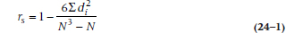
where d_i is the difference in ranks of a particular subject on the two measures. In the fourth column on Table 24–1 we have taken the liberty of doing this complex calculation for you. The sum of the squared differences looks like:

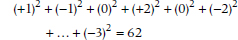
So the Spearman rank correlation is:

Because the formula came directly from the one for the Pearson r, it stands to reason that it equals .89, which is what we found earlier. Note that this does not mean that the two correlations always yield identical results. When both are calculated on ranked data (as in this case), they give the same answer. However, if the original data can be analyzed with a Pearson correlation (normality and all that other stuff), then converting these interval-property data to ranks results in the loss of information, and rho is lower than, rather than equaling, r.

We haven’t dealt with the issue of tied ranks, which is an inevitable consequence of using real data, something that has not yet constrained us. Our resource books tell us that, if the number of ties is small, we can ignore them. If it is large, we must correct for them.³ The formula involves messy corrections to both numerator and denominator of the Spearman formula using the number of ties in X and Y. We’ll let this one pass us by and let the computer worry about it.

The distribution of r_s is the same as that of Pearson’s r. The good news is that we don’t have to repeat how to calculate it; just refer back to Chapter 13 for all the gory details. The bad news is that you have to go through the same r to z‘ transformation to use the equations or Table P in the Appendix; and then convert the z‘ values back to rs.

TABLE 24–1 Ranking of moms on Amaze prowess and labor duration

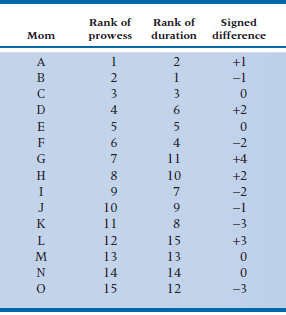
1 is highest proficiency; and 1 = briefest labor.

Significance of the Spearman Rho

We have already approached the issue of significance testing of a product-moment correlation. Because rho is so intimately related to the Pearson correlation, so is its significance test. It’s a t-test, yet again, where the numerator is the value of rho and the denominator is, as in Chapter 13, simply related to the value of rho and the sample size. So:

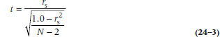
In this case, it equals:

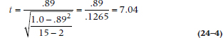
with df = N − 2, or (15 − 2) = 13. This value is, of course, wildly significant, so we can close up shop for the day.

We could stop there, but then Kendall (keep reading) would be left high and dry and would have to make his fame and fortune in motor oil. So, we’ll carry on a bit further.

THE POINT-BISERIAL CORRELATION

Just to ensure that you have a well-rounded statistical education, we will briefly mention another quaint historical piece, derived simply for simplicity in calculation. The point-biserial correlation was used in the situation were one variable was continuous and the other was dichotomous.⁴ For example, does any association exist between gender (two categories) and height (continuous)? It was calculated by starting with the Pearson formula, inserting a 1 and 0 for one variable, and then simplifying the equation. The resulting form is:

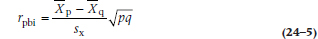
TABLE 24–2 Ranking of moms on Amaze prowess and labor duration

where p is the proportion of individuals with a 1, q is (1 – p), and s_x is the SD of the scores. Because the same result can be obtained simply by stuffing the whole lot—ones, zeros, and all—into the computer and calculating the usual Pearson correlation, there is little cause for elevating this formula to special status.

However, this formula is still applied with great regularity in one situation. In calculating test statistics for multiple choice tests, one measure of the performance of an individual item is the discrimination—the extent to which persons who perform well on the rest of the test and get a high score (the continuous variable) pass the item (the dichotomous score), and vice versa. This index is regularly calculated with (or at least expressed as) the point-biserial coefficient.

KENDALL’S TAU

Kendall created two approaches to measuring correlation among ranked data. The first, called tau (yet another Greek letter with no meaningful interpretation), generally underestimates the correlation when compared with other measures, such as rho.

Calculation of Tau

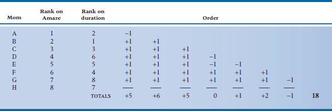
The calculation involves a bit of bizarre counting, but no fancy stuff. To get the ball rolling, we have copied the data of Table 24–1 into a new Table 24–2. The new table, however, has two changes. First, all the ranks of prowess are in “natural” order (i.e., from lowest to highest). They started out that way in Table 24–1, so we didn’t have to do anything. But if they hadn’t, this would be the first step. The second part is that we have copied only the first eight moms; this is for both our sanity and yours, as you shall soon see.

Once we have ordered one of the variables in ascending ranks and placed the ranks of the second variable alongside, the game now shifts entirely to the second variable. We start at each rank of this variable and count the number of occasions in which subsequent ranks occur in natural (i.e., ascending) order (add 1) or reversed (subtract 1) order. So looking at the first rank, 2, it is followed by a 1, which is in the wrong order, and therefore contributes a –1 to the running total. It is then followed by 3, 6, 5, 4, 8, and 7, all of which are greater than 2, so all contribute +1s to the total. We then go to the next rank in the durations, 1, and find (naturally) that all subsequent ranks—3, 6, 5, 4, 8, and 7—are in the right order, so this column contributes six +1s to the total. And so it goes, and eventually we end up with a total of +18. Clearly this method could drive you bananas if you had more than about 10 cases, but then no one ever said that this stuff was easy.

Now then, what’s going on? If no association existed between the two ranks, then (1) the second row of numbers would be distributed at random with respect to the first, (2) there would be as many –1s as +1s, and (3) the total would come out to zero. Conversely, if a perfect relationship existed, all the ranks on the second variable would be in ascending order, and because there are N(N – 1) ÷ 2 comparisons, the running total would be N(N − 1) ÷ 2 +1s—in this case, 28.

This then leads to the final step in the calculation. You take the ratio of the total to N(N − 1) ÷ 2 and call it “tau.”

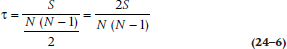
where S is the sum of the +1s and –1s. In our example, tau is equal to 18 ÷ 28 = .64. This is a whopping lot less than the Spearman correlation, but, of course, we deleted the last seven cases. Never fear, your intrepid authors took a night off to calculate the ruddy thing. The total S is 71, and the maximum is 15(14) ÷ 2, so tau is equal to 71 ÷ [15(14) ÷ 2] = .68.⁵ This is still substantially lower than the Spearman rho of .89 (we’ll see why in just a minute). We will go the last step, however, and see if it is significant anyway.⁶

TABLE 24–3 Ranking of orthopedic surgeons by three judges

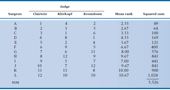
1 = highest rank on proficiency.

Significance Testing for Tau

As usual, significance testing involves constructing a t-test whose numerator is the coefficient itself and whose denominator is the SD of the coefficient. (Actually the numerator is [tau − 0] because we are trying to see if it differs from 0.) These SDs are really messy to derive and are the one place where real statisticians (unlike ourselves) earn their bread, so we’ll just take the answer on faith:

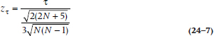
We have one small caveat; it doesn’t work for samples of less than 10, and, of course, only a fool would try to calculate τ for samples greater than 10. However, tables are around for looking up these SDs directly, including, of course, the proverbial bible of nonparametric statistics, Siegel and Castellan (1988). Tau has one redeeming quality; you can use it to calculate a partial correlation coefficient (the correlation between X and Y, controlling for the effect of Z). It is calculated in exactly the same manner as any other partial correlation (see Chapter 14). However, as we can never recall seeing it done, this is probably of marginal benefit.

Interpretation of Rho versus Tau

Both rho and tau are often presented as alternative ways of calculating the correlation between ordinal variables. But, there’s an important difference between them. Spearman’s rho is interpreted just like the Pearson correlation: square its value, and you’ll find the proportion of variance in one variable accounted for by the other. Kendall’s tau, though, is a probability—the difference between the probability that the data are in the same order versus the probability that they’re not in the same order. That means that if you run both on the same data, you’ll get different results, as we’ve just seen. As a rough approximation, tau × 1.33 = rho, and rho × 0.75 = tau.

KENDALL’S W

Not surprisingly, even Kendall had the good sense to figure that this one would be unlikely to put him in the history books. On the other hand, all the measures to date for ordinal data are like the Pearson correlation, in that they are limited to considering two variables at a time. It would be nice, particularly after learning the elegance of the intraclass correlation coefficient, if you could use an equivalent statistic for ordinal data.

Calculation of W

Remember the Olympic gymnastic championships, where emaciated little nymphettes paraded their incredible prowess in front of the judges while their doting mothers watched entranced from the sidelines? Remember the finale, where a bunch of 9.4 – 9.5 − 9.4 scores appeared magically across the TV screen? One score, from the home country, was always a bit higher, and one (from the communist or capitalist country, whichever was oppositely inclined politically), was lower.

Wouldn’t it be neat if we could do the same thing for surgery? Well, now we can! Welcome to the first annual Orthopedic Olympics. The surgeons are in the basement doing warm-up exercises, and the judges—Dr. Clairtete from McGill University in the country of Québec, Herr Dr. Prof. Klerkopf from Heidelberg, and Sam Kromdome from Hawvawd University—are in their booths. The first candidate presents herself and, in the flash of an eye, bashes off a double hip replacement, to the wild applause of all.⁷

After all 12 surgeons display their wares, the data look like those in Table 24–3. The fourth column shows the calculated average rank of each surgeon. So, the first sawbones rates (1 + 4 + 2) ÷ 3 = 2.33. Now, what would happen if the judges were in perfect agreement?⁸ The first would get a mean rank of (1 + 1 + 1) ÷ 3 = 1, and the last would get a rank of (12 + 12 + 12) ÷ 3 = 12. Conversely, if there were no agreement—a far more likely proposition—the rank of everybody would be about (6.5 + 6.5 + 6.5) ÷ 3 = 6.5. So the extent of agreement is related to the dispersion of individual mean ranks from the average mean rank. This is analogous to the intraclass correlation coefficient, where agreement was captured in the variance between subjects. It just remains to express this dispersion as a sum of squares, as usual, and then divide this by some expression of the max-imum possible sum of squares. The latter turns out to equal N(N² − 1) ÷ 12 (where N is the number of subjects), so Kendall’s W (the name of the new coef-ficient, for no reason we can figure⁹ equals:

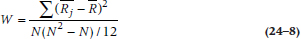
where and are mean ranks.

As with the formulae for the SD and other tests, this one is easy to understand conceptually but difficult computationally. We have to figure out the mean rank for each person, the overall mean rank, subtract one from the other, and so on, with rounding error introduced at each stage. An easier formula to use is:

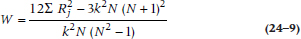
where R_j is the summed rank and k is the number of judges. It looks more formidable, but it’s actually quite a bit simpler to use.

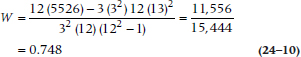
Backing up, we have calculated all the squared sums of the ranks in the far right column, which total up to 5,526. So W now equals:

Significance Testing for W

A simple approach for significance testing for W is available. If N is small (less than seven), you look it up in yet another ruddy table. For larger Ns, as it turns out (again for obscure reasons known to only real statisticians), a little jimcrackery on W gives you a chi-squared with (N − 1) df:

which in this case is:

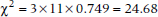
So in this case, the chi-squared is ridiculously significant.

GAMMA

Spearman’s rho and Kendall’s tau are used when we’ve rank ordered a large number of people, and it really doesn’t matter how many there are; we could be ranking five folks or 50. Sometimes, though, we’re dealing with a small number of ordered categories for two variables. For example, let’s say we grouped chiropractors into three categories according to how gentle or rough they are with their laying on of hands—Mothers’ Touch, Average, and Godzilla. We also have patients rate them in terms of how they feel afterwards—I Can Walk Again!, No Change, and Get Me Outta Here Now! The question is whether there’s a positive or negative relationship (or none) between these two variables.

Since there were still some Greek letters that hadn’t been used yet, Goodman and Kruskall thought, “Why don’t we use the letter gamma (Γ) and also invent a statistic that can deal with this situation? At the same time, let’s handle ties better than Spearman and Kendall do.” Gamma deals with ties in a most original way—it simply ignores them, and counts the number of pairs ranked in the same order by both raters or on both variables (N_s), and the number of pairs of cases that are ranked differently by both raters or on the two variables (N_D). Let’s see how it works.

To begin with, both variables have to be arranged in a table so that they go from highest to lowest. Just so we don’t have to use these long descriptors, we’ll call the best categories (Mother’s Touch and I Can Walk Again!) High; the worst categories (Godzilla and Get Me Outta Here Now!) Low; and the others Medium. In fact, there don’t have to be the same number of categories for the two variables, but we’ll stick with three for both of them. The pairs of ratings for 100 chiropractors each rated by one patient are shown in Table 24–4.

We next count how many pairs support the hypothesis that the two variables are positively related. We start in the upper left-hand cell (High-High, or HH if we want to be informal), and look at the cells that are to the right and below it. This includes the cells MM, ML, LM, and LL, and there are a total of 48 people in those cells. We then multiply 48 by the number of people in the HH cell (8), giving us 384, as we see in the first line of Table 24–5. Then we move on to the next cell, HM, and do the same thing (the second line in the table) and so on until we’re done. So, two questions—why those cells, and why did we multiply? Focusing just on the first line, any one person in HH is ranked higher on both variables than any person in the other cells in that row. Second, each of the 8 people in HH is higher than the 48 people in MM, so there are 384 pairs and so on for the other rows.

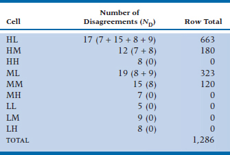
We now have to count up the number of pairs that go against our hypothesis; that is, where one person is higher than another on the first variable but lower on the second. The procedure is the same, but we now start with the upper right-hand cell (HL) and include the cells below and to the left, and we’ve summarized the results in Table 24–6.

After all that work, figuring out gamma is the easy part; it’s simply:

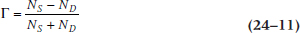
so in this case:

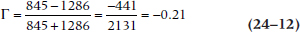
To figure out whether this is significant or not, we transform Γ into a z statistic:

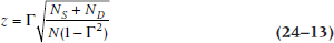
where N is the total number of pairs:

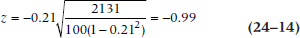
So, there’s a trend for Godzillas to be more effective than more gentle spine crackers, but it’s not significant.

WHAT WE’RE NOT TELLING YOU

We’re now going to tell you about two tests that we’re not going to tell you about. The point-biserial correlation is used (or at least, was used, before computers took over the world) when one variable is continuous and the other is naturally dichotomous, such as sex, or alive/dead. Sometimes, though, much against our sternest advice (Streiner, 2002a), the dichotomous variable is one that is naturally continuous, but has been split in two, such as dividing people into hypertensive/normotensive or euthymic/ depressed. In this case, the statistic to use is the biserial correlation, rather than the point-biserial. But, in our collective memories,¹⁰ we can’t recall a single time it has been used. Also, the point-biserial r is always smaller than the biserial r, so the bias is a conservative one.

The other correlation based on a 2 × 2 table we won’t mention is the tetrachoric correlation; not because it isn’t useful (it is), but because it’s next to impossible to figure out by hand. It’s a natural extension of the progression from the point-biserial (one dichotomous, one continuous variable) to the biserial (one dichotomous, one dichotomized continuous variable); the tetrachoric correlation is used when both variables are continua that have been dichotomized. The place where it is used most widely is when dichotomous items are being factor analyzed (a topic we discussed in Chapter 19). Fortunately, computers can do the work for us, so it’s sufficient to know it exists.

TABLE 24–4 Ratings of 100 Chiropractors in Terms of Touch and Effectiveness

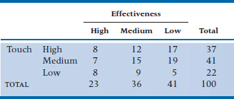
TABLE 24–5 Number of Agreements in Table 24–4

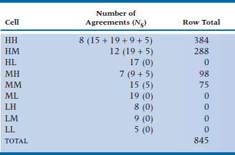
TABLE 24–6 Number of Disagreements in Table 24–4

There’s another reason we’re not telling. Like a lot of things in statistics, they carry the heavy weight of history on their shoulders; in this case, the history of hand calculations. For either one, if you simply took the formula for the Pearson correlation, made one or both of the variables dichotomous, and fiddled about with algebra, you would end up with the simplified (sort of) formulas we’re not showing you.

SUMMARY

That completes our little tour of agreement measures for ranked data. The most common by far is the Spearman correlation, rho, which is a reasonable alternative to the Pearson correlation. The advantage of Kendall’s W is that it can be used for multiple observers and thus is analogous to the intraclass correlation and is useful for agreement studies. Gamma is useful if we’re looking at agreement between two ordinal variables that have a limited number of categories. As far as tau is concerned, the less said, the better.

EXERCISES

1. For the following designs, indicate the appropriate measure of association:

a. Agreement between two observers on presence/absence of a Babinski sign.

b. Agreement between two observers on knee reflex, rated as 0, +, ++, +++, ++++.

c. Association between income of podia-trists and patient satisfaction (measured on a 7-point scale).

d. Agreement between two observers on religion of patients (Protestant, Catholic, Jewish, Muslim, Other).

e. Agreement among four observers on rating of medical-student histories and physical exams, using a 25-item checklist (both individual items and overall percent score).

f. Association between height and blood pressure.

g. Association between presence/absence of an elevated jugular venous pressure and car-diomegaly (present/absent on X-ray film).

h. Association between number of siblings and graduation honors.

i. Association between gender and graduation honors.

2. When any of us seek professional advice, whether from a plumber, mechanic, or statistician, our satisfaction is usually guided by the “three C’s”—correct, cheap, and cwick (sorry!).¹¹

Imagine a descriptive study of the association between time from initial contact with the statistician to the delivery of the analysis. To assess stability, each statistician is consulted twice, once with a simple problem and once with a hard one. Time from contact to delivery is measured in minutes, hours, days, or weeks, as appropriate. The data look like this:

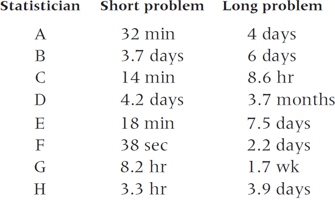
Analyze the data with the appropriate measure of association.

3. Evaluation of medical residents is notoriously unreliable. One way out of the swamp might be to get evaluators to rank individual residents, rather than rate them. Here are the results from a study involving ranking of 10 residents by (a) peers, (b) nurses, and (c) staff.

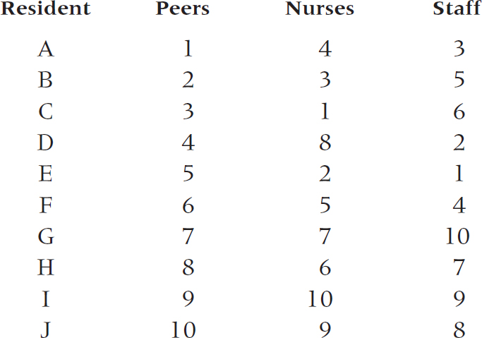
Analyze with the appropriate measure of association.

How to Get the Computer to Do the Work for You

Spearman’s rho

• 
  

  From Analyze, choose Correlate → Bivariate

  
  
• 
  

  Click the variables you want from the list on the left, and click the arrow to move them into the box labeled Variables

  
  
• 
  

  In the section named Correlation Coefficients, check the box to the left of Spearman

  
  
• 
  

  Click

Kendall’s tau

• 
  

  From Analyze, choose Correlate → Bivariate

  
  
• 
  

  Click the variables you want from the list on the left, and click the arrow to move them into the box labeled Variables

  
  
• 
  

  In the section named Correlation Coefficients, check the box to the left of Kendall’s tau-b

  
  
• 
  

  Click

Point-Biserial Correlation

• 
  

  Use Pearson’s r

Kendall’s W

• 
  

  From Analyze, choose Nonparametric Tests → K Related Samples

  
  
• 
  

  Click on the box for Kendall’s W

  
  
• 
  

  Note that, in order for this to work, the data must be rotated 90° to the way they appear in Table 24–3. Each judge is a subject, and each person rated is a variable.

Gamma

• 
  

  Afraid you’re out of luck. If you want to calculate it, you’ll have to do it by hand.

¹ One might speculate on the association between duration of labor and the driving status of husbands, as women never seem to deliver in their family cars.

² If you want to verify our calculations (always a good idea), Chapter 13 lists several forms of the Pearson correlation.

³ What they don’t say, of course, is how small is “small,” and how large is “large.”

⁴ Why did this coefficient end up in a chapter on ranked data? Because one variable is continuous, we couldn’t put it in Chapter 22. Because the other is categorical, we couldn’t put it in Chapter 13. So we averaged continuous and categorical and ended up here.

⁵ We invite you to check our calculations!

⁶ We will not bother with the corrections for tied ranks, as we see little point in using the ruddy things.

⁷ All except the son and heir, who hoped the old lady would croak.

⁸ We would all be absolutely incredulous, that’s what.

⁹ We do have a theory, however. Perhaps Kendall had (a) a lisp or (b) an Oriental mother, so that when he tried to say “R” it came out “AWA” and he just retained the W. (Yes, we know it’s farfetched.)

¹⁰ Which are admittedly getting shorter with each passing edition.

¹¹ Except for docs, because (a) you find out if they were wrong only after you die, (b) no doc is cheap, but then no one (hardly) pays for a doc out of his or her pocket anyway, and (c) you want the doc to be quick with everyone ahead of you and really slow with you.

Stay updated, free articles. Join our Telegram channel

Join