The Phi Coefficient, Contingency Coefficient, Yule’s Q and Cramer’s V

The most obvious approach is to pretend that the data are actually interval and go ahead and calculate a Pearson correlation. If the kid is identified by the psychologist as a troublemaker, he gets a “1,” if not, a “0”; if he ends up a YLC, he gets a “1,” if not, a “0.” And so we stuff 200 (x,y) pairs into the old computer, where each pair looks like (1,1), (1,0), (0,1), or (0,0), and see what emerges. As it turns out, this results in some simplifications to the formula. We won’t go through all the dreary details, but will just give you a glimpse. Remember that the numerator of the Pearson correlation was:

Now for the shenanigans. If we call the top left cell a, the top right one b, the bottom left c, and the bottom right cell d, then the first observation is that the sum of XY is equal only to a because this is the only cell where both X and Y are equal to 1. Second, the sum of X (the rows) is just (a + b), and the sum of Y is (a + c), again because this is where the 1s are located. Finally, N is equal to (a + b + c + d), the total sample size. The equation now becomes:

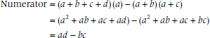
Similar messing around with the formula for Pearson correlation results in a simplication of the denominator, so that the final formula is equal to:

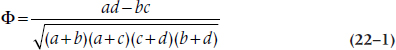
We have taken the liberty of introducing yet another weird little Greek symbol, which is called phi. The coefficient is, as you may have noticed from the title, the phi coefficient. For completeness, we’ll put the numbers in:

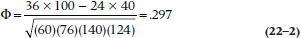
We’ll let you be the judge whether this correlation is high enough (or low enough) to merit trying to inspire a change in behavior.

Because the phi coefficient falls directly out of the 2 × 2 table, if the associated chi-squared is significant, so is the phi coefficient (and vice versa). In fact there is an exact relationship between phi and chi-squared:

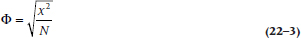
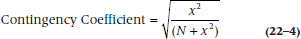
This relationship, and some variations, is the basis of several other coefficients. Pearson’s contingency coefficient, not to be confused with the product-moment correlation, looks like:

and in fact ϕ is the effect size (ES) indicator for the χ². However, there’s one problem with blindly using ϕ as an ES, and that is that its maximum value is 1 only when the row margins and the column margins are equal to 50%. In fact, the maximum possible value of ϕ for the data in Table 22–1 is 0.84.³ A better index of ES may be the ratio of ϕ to ϕ_Max, which, in this case, is .297 ÷ 0.84 and is a somewhat more impressive 0.35.

Cramer’s V is based on the chi-squared as well, but it is a more general form for use with I × J contingency tables. It is written as:

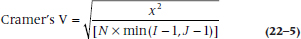
where the denominator means “N times the minimum of (I − 1) or (J − 1).” For a 2 × 2 table, this is the same as phi.

Both phi and V are interpreted as if they were correlations. So, if phi (or V) were equal to 0.50, then 25% of the variance (i.e., .50²) in one variable is accounted for by the other.

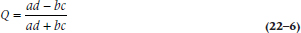
Yule’s Q is another measure based on the cross-product of the marginals, and it has a particularly simple form:

Choice among these alternatives can be made on cultural or aesthetic grounds as well as any other because they are all variations on a theme that give different answers, with differences ranging from none, through slight, to major.

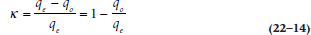
Cohen’s Kappa

A second popular measure of association in the biomedical literature is Cohen’s kappa (Cohen, 1960). Kappa is usually used to examine inter-observer agreement on diagnostic tests (e.g., physical signs, radiographs) but need not be restricted to such purposes. However, to show how it goes, we’ll create a new example.

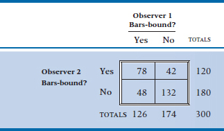
One clear problem with our above study is that we were left with a number of prediction errors, which may be due either to individual psychologists’ inability to agree on their predictions (an issue of reliability); or because they may agree based on the evidence available at the school, but this evidence is simply not predictive of future behavior (an issue of validity). Disagreement among observers will reduce the association, so it might be useful to examine the extent of agreement on this classification. This is straightforward. We assemble the files for a bunch of kids (e.g., n = 300), and get two psychologists to independently classify each kid as rotten or not. We then examine the association between the two categorizations, which are displayed in a 2 × 2 table, as in Table 22–2.

We could use phi here; however, kappa is a more popular choice as a measure of agreement in clinical circles for reasons that are likely more stylistic than substantive. To begin, let’s take a closer look at the data. How much agreement would we expect between the two shrinks just by chance? That is, if the psychologists don’t know beans about the students’ behaviors, they would still agree with each other a number of times, just by chance. Thus, the proportion of agreements would be non-zero.

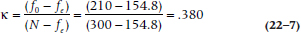
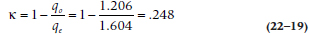
The chance agreement is calculated by working out the expected frequencies for the a and d cells, using the product of the marginals as we did with the chi-squared test. This equals (120 × 126 / 300) = 50.4 for cell a and (180 × 174 / 300) = 104.4 for cell d, for a total chance agreement of 154.8. Then we simply plug this expected frequency (f_e) and the observed frequency (f_o) for the two cells into the equation:

If you prefer to work with proportions, then divide each number by N (300 in this case), and use the formula:

where p_o is the observed proportion and p_e the expected.

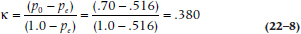
So, even though the observed agreement was a fairly impressive 70%, much of this was due to chance agreement, and the kappa is a less impressive .380.

Although kappa appears to start from a different premise than the phi coefficient, there are more similarities than differences after the dust settles. The numerator of kappa turns out also to equal (ad − bc), the same as phi. The denominators are different, but this amounts to a scaling factor. In fact, in this situation, phi is also equal to .380.

Standard error of kappa and significance test. To test the significance of kappa, it is first necessary to derive the standard error (SE; or the variance) of kappa, assuming that it is equal to zero. In its most general form, including multiple categories and multiple raters, this turns out to be a fairly horrendous equation. However, for a 2 × 2 table, it is a lot easier:

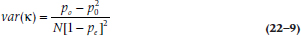
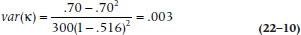
In the present case, p_o is .70, p_e is .516, and N is 300, so the variance equals:

TABLE 22–2 Inter-rater agreement on criminal status

Once the variance has been determined, the significance of kappa can be determined through a z-statistic:

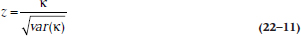
which in this case equals 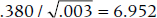—which is significant. In turn, the confidence interval about kappa is just 1.96 times the square root of the variance, or ± .107.

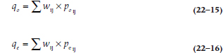
A problem with (and possible solution to) kappa. In Table 22–2, both observers were saying that roughly the same proportion of kids were destined to wear those unfashionable black-and-white striped pajamas (42% for Observer 1, 40% for Observer 2). We encounter a problem with kappa when the proportions between raters or between a rater and a measurement scale differ considerably. For example, let’s say that Observer 1 believed that most kids could be redeemed and that only 10% of the most serious cases were prison-bound⁴; while Observer 2 is a tough-nosed SOB, who foresees redemption in only 50%. We could conceivably end up with the situation shown in Table 22–3, where they both evaluate 100 cases. Cell a can’t have more than 10 people in it, nor can cell d have more than 50 because of the marginal totals.

TABLE 22–3 When the observers have very different assignment probabilities

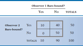
The raw agreement is 0.60, and kappa is a paltry 0.20. But let’s look at this table another way. Of all the cases who Observer 1 said were destined for the big house, Observer 2 agreed; and similarly, of all the people Observer 2 said were bound for jail, Observer 1 agreed. So, that kappa of 0.20 seems like a gross underestimate of how much they come to the same conclusion. For this reason, Loeber and Dishion (1983) introduced a variant of kappa called Relative Improvement Over Chance (RIOC)⁵ that compensates for the difference in base rate between the two observers (or an observer and a measurement tool). The simplified equation⁶ (Copas and Loeber, 1990) is:

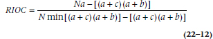
where min means the smaller value of (a + c) or (a + b). So, in this case, it becomes:

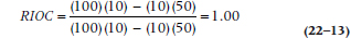
indicating that there is as much agreement as the differences in the marginal totals allow.

Things are rarely this extreme, but even so, that’s quite a difference—0.20 versus 1.00. So, which is right? In our (not so) humble opinion, neither kappa nor RIOC; the former is too conservative when the marginal totals are unequal, and the latter too liberal by not “penalizing” the observers for being so discrepant regarding their base rates. We’d be tempted to report both and let the readers see the table.

Generalization to multiple levels and dimensions. Kappa, unlike phi, can be generalized to more complex situations. The first is multiple levels; for example, we might have decided to get the counselors to identify what kind of difficulty the kids would end up in violent crimes, “white collar” crimes, drugs, and so on. Kappa can be used; it is just a matter of working out the expected agreement by totaling all the cells on the diagonal, then the expected agreement by totaling all the expected values, obtained by multiplying out the marginals. The ratio is then calculated according to the above formula.

Kappa can also be used for multiple observers, which amounts to building a 2 × 2 × 2 table for three observers, a 2 × 2 × 2 × 2 table for four observers, and so on. You can still work out the observed and expected frequencies on the diagonal (only this time in three-dimensional or four-dimensional space) and calculate the coefficient. Beware, though, that this is now a measure of complete agreement among three, four, or more observers and ignores agreement among a majority or minority of observers.

Finally, kappa can be used for ordinal data, without resorting to ranking. For this, we go to the next section.

PARTIAL AGREEMENT AND WEIGHTED KAPPA

Let’s continue to unfold the original question. In the first analysis, we found a relatively low and non-significant relationship between the prediction and the eventual status. In the next analysis, we explored the agreement on observer rating of criminal tendencies, which was only moderate. One way we might improve agreement is by expanding the categories to account for the degree of criminal tendency. Criminality, like most biomedical variables (blood pressure, height, obesity, rheumatoid joint count, serum creatinine, extent of cancer),⁷ is really on an underlying continuum. Shoving it all into two categories throws away information.⁸ We should contemplate at least four categories of prediction, for example “Saintly,” “Slightly Crooked,” “Street Thug,” and “Serial Killer.” If we again employ two observers, using the same design, the data would take the form of Table 22–4.

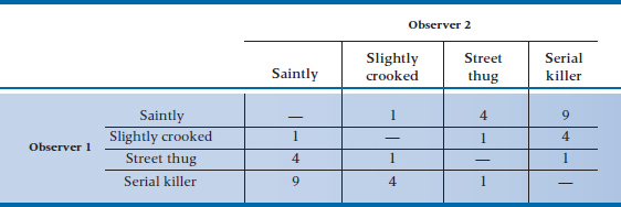
TABLE 22–4 Inter-rater agreement on criminal status

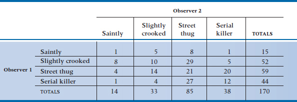
The first thing to note is that the overall agreement, on the diagonal, is now 44 ÷ 170, or 26%, which is pretty awful. If we went ahead and calculated a kappa on these data, using the previous formula, it would be less than zero. But there is actually a lot of “near agreement” in the table; 103 additional observations (8 + 14 + 27 + 5 + 29 + 20) agree within one category; combining these would yield an agreement of (44 + 103) ÷ 170 = .865, which is much better. The challenge is to figure out some way to put all these instances of partial agreement together into some overall measure of agreement.

Cohen (1968) dealt this problem a body blow with the idea of a weighted kappa, whereby the cells are assigned a weight related to the degree of disagreement. Full agreement, the cells on the diagonal, are weighted zero. (This does not mean that these very important cells are ignored. Stay tuned). The weights on the off-diagonal cells are then varied according to the degree of disagreement. The weights can be arbitrary and assigned by the user. For example, we might decide that a disagreement between Slightly Crooked and Street Thug is of little consequence, so this disagreement gets weighted 1; a difference between Saintly and Slightly Crooked gets a weight of 2; and a difference between Serial Killer and Street Thug is as severe as any of the greater disagreements (e.g., Serial Killer and Saintly) and all get weighted 4. We might do that—but we had better marshal up some pretty compelling reason why we chose these particular weights because the resulting kappa coefficient will not be comparable with any other coefficients generated by a different set of weights. (There is one exception. If the sole reason is to do comparisons within a study—for example, to show the effects of training on agreement—this is acceptable.)

The alternative is to use a standard weighting scheme, of which there are two: Cicchetti weights, which apparently are used only by Cicchetti (1972); and quadratic weights, which are used by everybody.⁹ For obvious reasons, we focus our attention on the latter. Actually the scheme is easy—the weight is simply equal to the square of the amount of disagreement. So, cells on the diagonal are weighted 0; one level of disagreement (e.g., Serial Killer vs Street Thug) gets a weight of 1²= 1; two levels of disagreement (e.g., Serial Killer vs Somewhat Crooked) gets weighted 2² = 4, and so on up.

To see how this all works, we begin with the formula for kappa, in Equation 22–8, and then substitute q = (1 − p) for everything. In other words, the formula is rewritten in terms of disagreement instead of agreement. The revised formula is now:

It is now a matter of incorporating the various weighting schemes into the q’s. No problem—just sum up the weighted disagreements, both observed and expected (by taking the product of the related marginals divided by the total), over all the cells (i,j), which are off the diagonal: where w_ij are the weights for the cells. These are then popped back into the original equation, and that gives us weighted kappa.

To demonstrate how this all works, let’s calculate the example in Table 22–4. In Table 22–5, we have worked out the expected frequencies by taking the product of the marginals and dividing by the total. (Note that we did this calculation only for the off-diagonal cells. Why make work for ourselves when we don’t use the data in the diagonal cells?) In Table 22–6, we have shown what the quadratic weights for each cell look like.

Now we can put it all together. Keep in mind that the tables show the frequencies and we need the proportions, so we will have an extra “170” kicking around in the summations. Now the observed weighted disagreement, going across the rows and then down the columns, is:

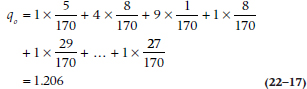
TABLE 22–5 Expected frequencies for rater agreement

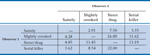
TABLE 22–6 Quadratic weights for rater agreement

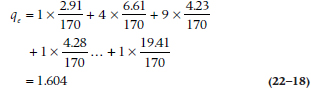
and the expected weighted disagreement is:

So the weighted kappa in this case is:

Although this is not terribly impressive, it is an improvement over the unweighted kappa for these data, which would equal −.018. The general conclusion is that the weighted kappa, which takes partial agreement into account, is usually larger than the unweighted kappa.¹⁰

RELATION BETWEEN KAPPA AND THE INTRACLASS CORRELATION

One reason Cicchetti was fighting a losing battle is that the weighted kappa using quadratic weights has a very general property—it is mathematically (i.e., exactly) equal to the ICC correlation. We must be pulling your leg, right? Nope. We know that the ICC comes out of repeated-measures ANOVA (see Chapter 11) and is useful only for interval-level data, and kappa is based on frequencies and nominal or ordinal data.

But just suppose we didn’t tell the computer that. We call Saintly a 4, Slightly a 3, Street a 2, and Serial a 1. We then have a whole bunch of pairs of data, so the top left cell gives us one (4,4) and the bottom right cell gives us a total of 12 (1,1)s. There are, of course, 170 points in all. We then do a repeated-measures ANOVA where Observer is the within-subject factor with two levels. We calculate an ICC, just as we did in Chapter 11. The result is identical to weighted kappa. It also follows that, if we were to analyze a 2 × 2 table with ANOVA, using numbers equal to 0 and 1, unweighted kappa would equal this ICC when calculated like we did above (Cohen, 1968).

Who cares? Well, this eases interpretation. Kappa can be looked on as just another correlation, explaining some percentage of the variance. And there is another real advantage. If we have multiple observers, we can do an intraclass correlation and report it as an average kappa¹¹ instead of doing a bunch of kappas for observer 1 vs observer 2, observer 1 vs 3, etc.

SAMPLE SIZE CALCULATIONS

Sample size calculations for phi, kappa, and weighted kappa are surprisingly straightforward. To test the significance of a phi coefficient (i.e., to determine whether phi is different from zero), we simply use the sample size formula for the equivalent chi-squared because both are based on the same 2 × 2 table. This was outlined in Chapter 21, so we won’t repeat it.

For kappa, you must first consider a bit of philosophical decision making. If the point of the study is to determine whether kappa is significantly different from zero, we can use the formula in Equation 22–9 to derive an SE for kappa and then insert this into the usual formula for sample size:

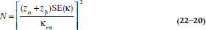
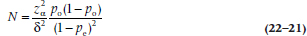
where κ_est is the estimated value of kappa. However, this philosophical stance presumes that a kappa of zero is a plausible outcome. If you are looking at observer agreement, an agreement of zero is hopefully highly implausible (although it happens only too often). In this case, you are really hoping that your estimate of the agreement is somewhere near the true agreement. In short, you want to establish a confidence interval around your estimated kappa. The formula for the SE of kappa (Equation 22–9 again) is a likely starting point, and it is necessary only to decide what is a reasonable confidence interval, δ (say, .1 on either side of the estimate, or .2), then solve for N. Of course, the fact that you have to guess at the likely value for both p_o and p_e in these equations gives you lots of freedom to come up with just about any sample size you want. The formula is now:

The sample size for weighted kappa would require too many guesses, so a rule of thumb is invoked: the minimum number of objects being rated should be more than 2c², where c is the number of categories (Soeken and Prescott, 1986; Cicchetti, 1981). So in our example, with four categories, we should have 2 × 4² = 32 objects.

SUMMARY

This chapter has reviewed three popular coefficients to express agreement among categorical variables. The phi coefficient is a measure of association directly related to the chi-squared significance test. Kappa is a measure of agreement particularly suited to 2 × 2 tables; it measures agreement beyond chance. Weighted kappa is a generalization of kappa for multiple categories, used in situations where partial agreement can be considered. Unless there are compelling reasons, weighted kappa should use a standard weighting scheme. When quadratic weights are used, weighted kappa is identical to the intraclass correlation, which was discussed in Chapter 11.

EXERCISES

1. Consider a study of inter-rater agreement on the likelihood that psychiatric patients have von Richthofen’s disease (VRD, characterized by the propensity to take off one’s shirt in the bright sunlight—the “Red Barin’ Sign”). Two psychiatrists indicate whether or not patients have VRD, rated as Present or Absent.

Suppose we now did a second study where they did the same rating, only this time on a four-point scale, from “Definitely Present” to “Definitely Absent.” What would happen to the following quantities?

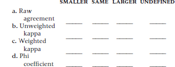
2. The following 2 × 2 table displays agreement between two observers on the presence or absence of the dreaded “Red Barin’ Sign” (see above for explanation):

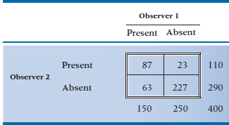
Calculate

a. Phi

b. Contingency coefficient

c. Cramer’s V

d. Cohen’s kappa

How to Get the Computer to Do the Work for You

Phi and Kappa

• From Analyze, choose Descriptive Statistics → Crosstabs
  
• Click on the variable you want for the rows and click the arrow to move it into the box labeled Row(s)
  
• Do the same for the second variable, moving it into the Column(s) box
  
• Click the button and choose Phi and Cramer’s V and/or Kappa, then
  
• Click

¹ Who can forget Goodman’s Gamma and Lambda or Somer’s d? We can, and so can you.

² We could also treat this as a screening test for YLC (“If the test is positive, it’s highly likely that the kids will end up in the can”) and determine the sensitivity (36 ÷ 76 = .47), specificity (100 ÷ 124 = .81), positive predictive value (36 ÷ 60 = .60), and negative predictive value (100 ÷ 140 = .71). We could but we won’t—this is a statistics book. For more details see PDQ Epidemiology.

³ If you want to know how we figured out that little bit of legerdemain, we kept the marginal totals the same, put all of the cases in cell B into cell A, which maximizes the association, and then redid the χ².

⁴ Obviously, a psychologist who switched from social work.

⁵ Ironically, in a paper devoted to the prediction of male delinquency.

⁶ Believe us; this is the simplified version.

⁷ We used to think that the only real dichotomous variables were pregnancy and death. However, with life-support technology, death is now up for grabs.

⁸ For an elaboration, see Health Measurement Scales: A Practical Guide to Their Development and Use (Streiner and Norman, 2014).

⁹ Strictly speaking, the formula is (Everybody − 1); Cicchetti doesn’t.

¹⁰ It is also a general, although counterintuitive, finding that increasing the number of boxes on the scale will improve reliability, as assessed by weighted kappa or an ICC correlation, even though the raw agreement is reduced. For an elaboration, see Streiner and Norman (2014).

¹¹ This also accommodates apparently religious differences among journals. Some journals like ICCs, some like kappas. We have, on occasion, calculated an ICC and called it a kappa, and vice versa, just to keep the editor happy.

Stay updated, free articles. Join our Telegram channel

Join