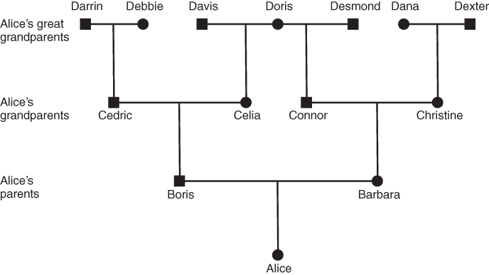
Figure 3.2 Genealogy of an inbred reference person (Alice) going back three generations. Squares indicate males; circles, females. Horizontal lines indicate matings, and vertical lines indicate descent from these matings. Note that in this example, Alice has only seven great grandparents (compared with eight in Figure 3.1). Alice’s father’s mother’s mother is the same as her mother’s father’s mother (Doris). This makes Alice’s parents (Boris and Barbara) half first cousins, because they share one grandparent (Doris).

As noted in the previous chapter, Hardy–Weinberg equilibrium assumes that all mating is random and that two mates are completely unrelated; in other words, no inbreeding. We can see that this will never be strictly true, as we are all related and inbred to some extent. However, the genetic impact of inbreeding depends on the closeness of the relationship of the parents. If two parents are seventh cousins, then the degree of relationship is so small that for all practical purposes they are unrelated. More significant deviations from the assumption of random mating are associated with close degrees of relationship, such as mating between siblings, uncles and nieces (or aunts and nephews), or first cousins.

In addition, as noted earlier, inbreeding does not directly change the frequency of an allele, and is therefore not an evolutionary force. Instead, inbreeding changes the genotype proportions from those expected under Hardy–Weinberg equilibrium, such that the frequency of homozygotes is increased, and the frequency of heterozygotes is decreased. Although inbreeding by itself does not change allele frequencies, it can interact with one of the evolutionary forces to change the rate of allele frequency change. As an example (to be covered in more detail in Chapter 6), imagine a case where there is selection against a recessive homozygote. Under inbreeding, there will be a greater number of these homozygotes with each generation such that a greater proportion of the population will be selected against, and the speed of selection will therefore be greater than under Hardy–Weinberg equilibrium. Again, the exact impact of inbreeding relative to random mating will depend on the level of inbreeding.

This chapter begins with the concept of the inbreeding coefficient (a measure of the level of inbreeding) and how inbreeding is determined from genealogical data. This introduction is followed by an explanation of how inbreeding affects genotype frequencies but not allele frequencies. This chapter concludes with discussion of variation in rates of inbreeding in human populations as well as several case studies of measurement and analysis of inbreeding in human populations. Inbreeding is of particular interest in studies of human population genetics because different cultures may have different rules and preferences for and against different levels of inbreeding. The study of inbreeding in human populations thus provides an opportunity to examine how human culture affects genetic variation.

3.1 Quantifying Inbreeding

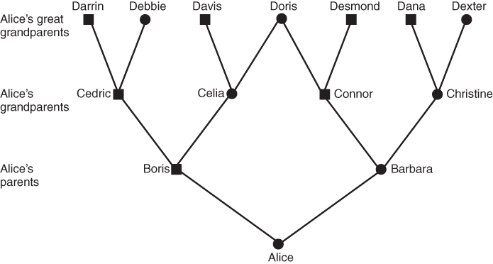
Genealogical diagrams provide the best way to understand common ancestry and inbreeding. There are several different ways of drawing genealogies, with different symbols used to designate males and females, and different arrangements of lines to illustrate lines of descent. How would you draw your family tree back three generations? One way of doing this has already been shown in Figures 3.1 and 3.2, with horizontal lines indicating matings and vertical lines to indicate descent. Another method is shown in Figure 3.3, depicting the same relationships as in Figure 3.2 but eliminating the horizontal lines and using diagonal lines to indicate descent. This method is used throughout this text because it is easier to see descent and genetic relationships when discussing inbreeding.

Figure 3.3 Genealogy of an inbred reference person (Alice) going back three generations. Squares represent males; circles, females. This diagram shows the same inbreeding relationship as in Figure 3.2, but diagonal lines are used to indicate descent from pairs of parents. Although the system used in Figures 3.1. and 3.2 is often preferred in genealogical illustration, the system of diagonal lines is used throughout the text, as it is easier to convey descent and genetic inheritance.

Because our focus here is on genetic relationships, all of the hypothetical genealogies used here refer to mating (a biological act) and not marriage (a culturally defined relationship). Although anthropologists and geneticists will sometimes use marriage records to reconstruct genealogies, we have to keep in mind the possibility that some births result from extramarital relationships. Likewise, a genealogy based on cultural definitions of family and kinship could include relationships that were established through adoption or remarriage (stepparents), which would not indicate an actual genetic relationship. Unless otherwise noted, all discussions of inbreeding here refer to one’s biological relatives.

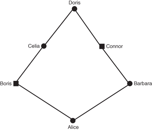
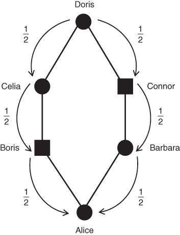
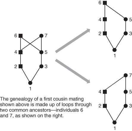
Figures 3.2 and 3.3 both show an inbred person whose parents are half first cousins. The nature of inbreeding is very clear from Figure 3.3. In any genealogy, a person is inbred if you can draw a line back through to a common ancestor and then back to the original person through a different line. In other words, a person is inbred if you can draw a loop back through one or more common ancestors. This loop is even clearer in Figure 3.4, which takes Figure 3.3 and eliminates those ancestors who are not part of the inbreeding loop. Figure 3.4 shows the loop as starting with Alice and then going backward three generations to the common ancestor (Doris). The complete loop is Alice–Boris–Celia–Doris–Connor–Barbara–Alice.

Figure 3.4 Genealogy of an inbred person (Alice) showing only the lines of descent that contribute to inbreeding (all other individuals are not shown). This figure is the same as Figure 3.3 after eliminating all ancestors who are not involved in the inbreeding. As shown here, the nature of inbreeding as a “loop” of ancestry is clear. The complete loop is Alice–Boris–Celia–Doris–Connor–Barbara–Alice.

3.1.2 Types of Inbreeding

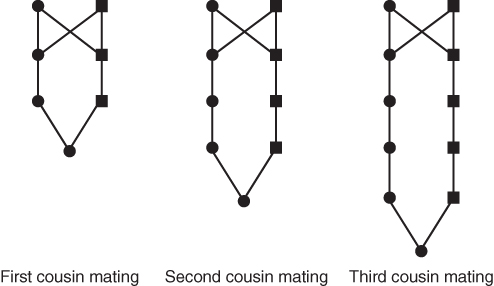
We can use this simplified form of genealogy, showing only ancestors in the chain of inbreeding, to illustrate different types of inbreeding. Extremely close forms of inbreeding occur with the offspring of parent–child mating, sib mating, and half-sib mating, all of which are shown in Figure 3.5. Different types of cousin marriage are shown in Figure 3.6. Cousins are referred to by number—first, second, third, and so on—which refers to the depth of the relationship. First cousins share one or more grandparents; the diagram in Figure 3.6 shows full first cousins, who share two grandparents. Second cousins share great grandparents, and third cousins share great-great grandparents.

Figure 3.5 Diagrams of five types of close inbreeding. As in previous figures, only ancestors that are part of the loop through common ancestors are shown.

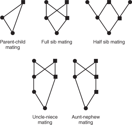
Figure 3.6 Diagrams of cousin mating. As in previous figures, only ancestors that are part of the loop through common ancestors are shown. First cousins share a set of grandparents, second cousins share a set of great grandparents, and third cousins share a set of great grandparents.

There are also variations on the different types of cousin marriages. As shown in Figure 3.7, “first cousins once removed” describes the relationship between a person and the child of their first cousin. The “removed” term refers to the number of generations apart the two cousins are separated; “once removed” is one generation apart, “twice removed” refers to two generations apart, and so on. It might be useful to think about your own family to understand the relationship between various cousins. If you have a first cousin, think of that person and the set of grandparents that you have in common with that cousin. If your cousin has a child, that child is your first cousin once removed. If you also have a child, your child and your first cousin’s child are second cousins. Likewise, if your second cousin has a child, that child is your second cousin once removed. If that child then has a child, your second cousin’s grandchild will be your second cousin twice removed. Yes, it can get very complicated quickly!

Figure 3.7 Diagrams of variations of first cousin mating. As in previous figures, only ancestors that are part of the loop through common ancestors are shown. Mating between first cousins once removed is between a person and the child of their first cousin, thus involving a mating between generations. First cousins share two grandparents, as shown in Figure 3.6. In half first cousin mating, only one grandparent is shared. In double first cousin mating, all four grandparents are shared. Note that half first cousin mating was already shown, albeit in somewhat different form, in Figures 3.3 and 3.4.

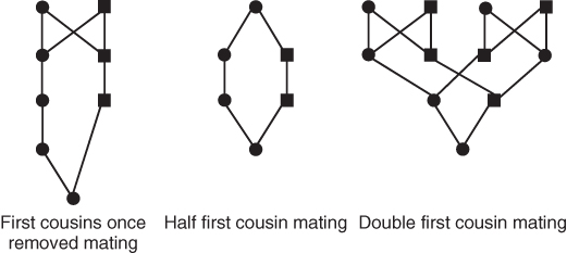
Figure 3.7 shows two other variations on first cousin mating. Whereas first cousins as shown in Figure 3.6 share two grandparents, half first cousins share only one grandparent (as was shown earlier in Figures 3.2 and 3.3). The last example in Figure 3.7 shows the mating between double first cousins. Two people are double first cousins if they share all of their grandparents. As shown here, picture two couples, each having a male child and a female child, and then having the brother and sister in one family mating with the brother and sister in the other family, producing double first cousins.

All of the matings shown in Figures 5–7 produce a child that is inbred, because all of these diagrams show a loop back through one or more common ancestors. Note that while it only takes one common ancestor to define a case of inbreeding, some types of mating involve more than one common ancestor, and thus we can draw more than one loop. For example, in Figure 3.6, full first cousin mating involves two common ancestors, and we could draw two loops, one for each grandparent. Half first cousin mating involves only one common ancestor, and we can draw only one loop. Double first cousin mating has four common ancestors (all of the grandparents), and we can therefore draw four loops (see Figure 3.7).

3.1.3 The Inbreeding Coefficient

We will now use the concept of inbreeding as a genealogical loop through one or more common ancestors to provide a quantitative measure of inbreeding known as the inbreeding coefficient. As noted in Chapter 1, homozygosity refers to the case where an individual has inherited the same allele from both parents. In the simple example of a locus with two alleles, A and a, the homozygous genotypes are AA and aa. Homozygosity is defined as the two alleles being identical, but there are actually two reasons why this identity can occur—identity by descent and identity by state. Identity by descent is when the two alleles are the same because they were both inherited from a common ancestor. Identity by state occurs when the identical alleles do not come from a common ancestor. The inbreeding coefficient (typically denoted by the symbol F) is the probability that an inbred individual has two alleles at a given locus that are identical because of inheritance from a common ancestor. F is thus the probability of identity by descent.

3.1.3.1 How to Compute the Inbreeding Coefficient

Figure 3.8 shows how this probability can be computed from the genealogy of an inbred individual. In this case, we are using the case of a person whose parents were half first cousins as was shown previously in Figures 3.3 and 3.4. The curved lines indicate the transmission of alleles from parent to child across the generations; in each case, the probability of a parent passing on a given allele to a child is . As described in the legend to Figure 3.8, the probability of Alice getting the A allele from both lines of descent from the common ancestor Doris is , and the probability of obtaining the a allele from both lines of descent is also . For Alice to have either homozygous genotype (AA or aa) is computed using the or rule, giving .

Figure 3.8 Genealogy of an inbred person (Alice) showing only the lines of descent that contribute to inbreeding (all other individuals are not shown). This is the same genealogy as in Figure 3.4. The curved arrows indicate the path of genetic descent with the associated probability of from parent to child. These probabilities allow us to compute the probability of Alice having a homozygous genotype (AA or aa) because of identity by descent. Imagine that the common ancestor (Doris) has the genotype Aa. The probability of her passing on the A allele to her daughter Celia is . The probability of Celia passing that A allele on to Boris is also , as is the probability of Boris passing it on to Alice. Thus, the probability of the A allele being passed on from Doris to Celia to Boris to Alice is computed using the and rule as . Now, for Alice to receive an A allele from the other line of descent from the common ancestor Doris, the probability of the allele being passed from Doris to Connor and from Connor to Barbara and from Barbara to Alice is also . In order for Alice to receive an A allele from both lines of descent from Doris is the probability of both events occurring, which is . We also have to consider the probability of Alice having the other homozygous genotype (aa) because of identity by descent, which would occur when Alice receives the a allele from both lines of descent from Doris. This probability would also be . Because the probability of Alice having the AA genotype because of identity by descent is , and the probability that Alice will have the aa genotype because of identity by descent is also , the probability of her having either the AA or the aa homozygous genotype is solved using the or rule as . Thus, .

An easier shortcut can be used here:

where i is the number of individuals that lie in the loop up through the common ancestor and then down again, not counting the inbred person. Referring to Figure 3.8, we can identify the ancestors that lie on the loop from Alice to Doris and back (not counting Alice) as Boris–Celia–Doris–Connor–Barbara. There are five people in this loop, so i = 5 and . Thus, the probability of Alice having a homozygous genotype (AA or aa) because of identity by descent is 0.03125.

Computation of F gets a little bit more complicated when there is more than one common ancestor, because we need to add up the probabilities over all possible paths of descent. Consider the case of first cousin mating shown in Figure 3.9. There are two common ancestors, numbered 6 and 7. We therefore need to consider two inbreeding loops. One loop is through ancestor number 6: 1–2–4–6–5–3–1. The other loop goes through common ancestor number 7: 1–2–4–7–5–3. We now compute the inbreeding coefficient for each loop, and then add them together. The method of dealing with more than one common ancestor can be summarized with the following formula:

3.1

The symbol ∑ is the uppercase Greek letter sigma, which is used in mathematics to sum whatever terms are to the right of the symbol. In this case, the summation is over the number of common ancestors. In Figure 3.9, there are two common ancestors—individuals 6 and 7. For ancestor 6, we have , because there are five ancestors in the loop through this ancestor. For ancestor 7, the value is also because there are five ancestors in the loop through ancestor 7. Using equation (3.1), the total inbreeding coefficient is therefore the sum of these, giving .

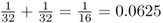Figure 3.9 Computing the inbreeding coefficient of first cousin mating. The genealogy on the left side represents the mating of first cousins (individuals 2 and 3). There are two common ancestors, labeled here as individuals 6 and 7. In order to compute the inbreeding coefficient for individual 1, we need to count the number of ancestors in each loop shown on the right side of the figure. For common ancestor 6, the number of ancestors in the loop (not counting individual 1) is i = 5. For common ancestor 7, the number of ancestors is also i = 5. Using equation (3.1), the inbreeding coefficient for a first cousin mating is .

3.1.3.2 Inbreeding Coefficients for Different Levels of Relationship

Table 3.1 presents inbreeding coefficients for various types of relationship ranging from parent–child through third cousin matings; most of the matings in Table 3.1 are shown in Figures 3.5, 3.6, 3.7. To make sure that you understand how to compute the inbreeding coefficient, you should try using equation (3.1) on the different genealogies in Figures 3.5, 3.6, 3.7 to see if you get the same values.

Table 3.1 Inbreeding Coefficients for Different Types of Mating

Mating	Inbreeding Coefficient) (F)
Parent–child
Full sibs
Half sibs
Uncle–niece/aunt–nephew
Double first cousins
First cousins
Half first cousins
First cousins once removed
Second cousins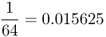
Second cousins once removed
Third cousins

Source: Data from Schull (1972).

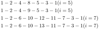
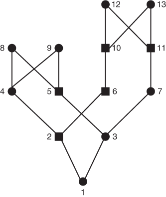
Keep in mind that inbreeding can also be cumulative when a person’s parents are related in more than one way. Figure 3.10 presents a genealogy where person 1 is inbred because her parents (individuals 2 and 3) are simultaneously first cousins and second cousins. Listing all possible loops of common ancestry and using equation (3.1), we compute the inbreeding coefficient of person 1 as F = 0.078125.

Figure 3.10 Example of a genealogy where the parents of an inbred person (individual 1) are both first and second cousins. As in previous figures, only ancestors directly in one or more loops of inbreeding are shown. The parents (individuals 2 and 3) are simultaneously first cousins (through ancestors 8 and 9) and second cousins (through ancestors 12 and 13). In order to compute the inbreeding coefficient, we need to tally the number of ancestors (i) in each possible loop through a common ancestor. The loops and number of ancestors in each loop are as follows:

Using equation (3.1), we can now sum up the quantity over all loops, giving .

Stay updated, free articles. Join our Telegram channel

Join