2.1 Genotype And Allele Frequencies

Before getting into the definition, derivation, and application of Hardy–Weinberg equilibrium, some basic ideas for measuring genetic variation in a population need to be clarified, specifically the ideas of genotype frequencies and allele frequencies.

2.1.1 Computing Genotype Frequencies

Once again, we use the standard model of a hypothetical locus with two alleles, A and a. As covered in the previous chapter, when we have two alleles, we will have three genotypes: AA, Aa, and aa. To make things easy, let us suppose that the two alleles are codominant, so that we can tell the difference between people having these three genotypes. Imagine that we visit a population and test the genotype of 150 people, and obtain the following numbers:

The first thing we would want to do is to figure out the genotype frequencies, which are the proportions of each genotype. To do this, we simply divide each number by the total number of individuals. Thus, because 54 of 150 people have the AA genotype, the genotype frequency is . We can do this for all three genotypes:

Although it might seem obvious, it will be important later to see that the sum of the genotype frequencies adds up to 1 (0.36 + 0.48 + 0.16 = 1.0). Although we use genotype frequencies in population genetics, note that we could also express these proportions as percentages by multiplying each proportion by 100: AA = 36%, Aa = 48%, and aa = 16%. Note that these add up to 100%.

At this point, it is useful to consider another characteristic of genotype frequencies. Suppose that you were to return to this population and choose a single person at random without knowing that individual’s genotype. What is the probability that this person would have the genotype AA? The answer is 0.36, which is the genotype frequency, because this number also represents the number of times that a specific event occurs (54 people have genotype AA) divided by the total number of events (there are 150 people).

2.1.2 Computing Allele Frequencies

You can see that it is easy to estimate out the relative frequency of any genotype; you simply divide the number by the total number of all genotypes. What about the frequency of an allele? What are the number of A alleles and the number of a alleles in the hypothetical population described above?

2.1.2.1 Two Alleles

The answer to these questions may not be immediately obvious. I have found that many students understand better the concept of allele frequency using an analogy. Imagine there are 150 people each wearing two socks (one on each foot). For reasons unknown to us (you are welcome to make one up), some of the people are wearing two black socks, some are wearing a black sock and a white sock, and some are wearing two white socks. Suppose that you count them up and come up with the following numbers:

Now, how many black socks are there in this group of people? If you rush in answering this question, you might come up with 126 people by adding the 54 people, with two black socks and the 72 people with one black sock, but that is actually the number of people having at least one black sock, which is not what I asked. Instead, you have to count the actual number of black socks, keeping in mind that some people are wearing two and some people are wearing only one. In this example, we have 54 people, each with two black socks, and 72 people with only one black sock. When we add these up, we get a total of

We can do the same thing for the number of white socks. We have 72 people with one white sock and 24 people with two white socks, giving a total of

We have 180 black socks and 120 white socks, for a total of 300 socks, which makes sense because we have a total of 150 people, each with 2 socks [ = 150(2) = 300]. We could now figure out the relative frequency of black socks by dividing the number of black socks by the total number of socks, which is . Likewise, the relative frequency of white socks is .

You probably noticed that the numbers I used in the genotype frequency example and the sock example are the same. This was done on purpose to enable you to extend the sock analogy to the concept of allele frequencies. The computation is the same, except that instead of counting socks you are counting alleles. Let us return to the original question. Given the genotype numbers AA = 54, Aa = 72, and aa = 24, what are the relative frequencies of the A and aalleles? Start by counting the number of A alleles, remembering to count the A allele twice for the AA genotype and once for the Aa genotype. There are 54(2) + 72(1) = 180 A alleles. We repeat this procedure for the number of a alleles, getting 72(1) + 24(2) = 120 a alleles. Thus, this hypothetical population has 180 A alleles and 120 a alleles for a total of 300 alleles (which works out since there are 150 people, each with two alleles). Therefore, the relative frequency of the A allele is , and the relative frequency of the a allele is . A simple way to keep all of these calculations straight is to make a table that lists the number of A alleles and the number of a alleles for each of the three genotypes, as shown in Example 2.1.

Example 2.1

How to Compute Allele Frequencies

In this example, we use the hypothetical example from the text of a single locus with two alleles, A and a. The data are

In the following table, we list the number of A and a alleles and the total number of all alleles for each genotype, and then sum each column:

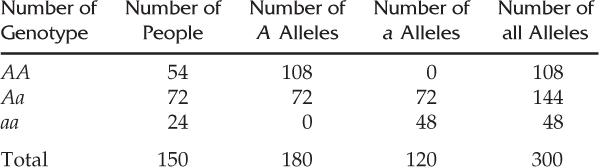
There are a total of 180 A alleles and 120 a alleles in this population, for a total of 300 alleles (twice the number of people sampled, because each person has two alleles).

As a check, the allele frequencies should add up to 1.0, which they do (0.6 + 0.4 = 1.0).

Because we use allele frequencies extensively in population genetics equations, we use symbols to refer to the different allele frequencies. Although you can feel free to create any symbol you wish, the conventional format is to use the symbol p to refer to one allele and the symbol q to refer to the other allele. In Example 2.1, p is the relative frequency of the A allele and q is the relative frequency of the a allele. We will use this notation throughout the rest of the book.

Note that in the case of two alleles, there are only two allele frequencies, and these numbers must add up to 1.0. In Example 2.1, this is seen because 0.6 + 0.4 = 1.0. This property allows us a convenient check on our math; if the two allele frequencies do not add up to 1.0 (or very close, in the case of irrational numbers and roundoff), then an error was made in computing the allele frequency. Beware—I have seen this error on homework assignments, so you should always take time to check your answers thoroughly.

Mathematically, we can express the sum of the allele frequencies using the following simple formula:

2.1

Note that this relationship allows us to predict one allele frequency if we know the other, because, using some simple algebra, we see that

2.2

These relationships may be intuitively obvious, but as you will see, they allow us to handle much of the mathematics of population genetics in an elegant manner.

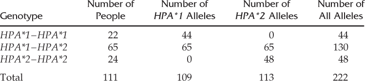
As another example of computing allele frequencies, I will use a real-world case. In the 1960s, anthropologist Jonathan Friedlaender collected data on a number of genetic markers of the blood in 18 villages on the island of Bougainville in Melanesia. One of the markers collected was the haptoglobin locus, a gene located on chromosome 16. This locus has two alleles, HPA*1 and HPA*2. In the village of Nupatoro, Friedlaender (1975) collected blood samples from 111 villagers, and found the following genotype numbers:

The genotype frequencies are obtained by dividing each number by the total number:

We find that there are 109 HPA*1 alleles and 113 HPA*2 alleles, for a total of 222 alleles (twice the number of people sampled). This gives allele frequencies for HPA*1 of and for HPA*2 of . The full computation is provided in Example 2.2 for review.

Example 2.2

How to Compute Allele Frequencies

This example is based on an actual study of human population genetics. Data on a number of genetic markers were collected by Friedlaender (1975) on Bougainville Island in Melanesia. One of these markers was the red blood cell protein haptoglobin protein, a locus with two alleles: HPA*1 and HPA*2. Genotype numbers and number of alleles are shown below:

2.1.2.2 More than Two Alleles

Much of population genetics theory builds on a simple model of a single locus with two alleles. In the real world, however, there are many loci (particularly DNA markers) with more than two alleles. How can we compute allele frequencies in such cases? For loci where all the alleles are codominant, allowing identification of each genotype, the answer is simple—we count the number of alleles in the same manner. Example 2.3 shows computations for a locus with three alleles. When we have three alleles, we typically label the allele frequencies as p, q, and r (when there are more than three alleles, it is common to simply use the letter p with a subscript to refer to different alleles).

Example 2.3

How to Compute Allele Frequencies for a Locus with Three Alleles

Salzano et al. (1985) collected data from 216 Pacaás Novos Indians of Brazil on the group-specific component locus (GC, also known as the vitamin D binding protein) on chromosome 4, which codes for a protein. A number of early studies indentified two alleles, GC*1 and GC*2, but later work identified two subtypes of the GC*1 allele, known as GC*1F and GC*1S. Salzano et al. collected data on the six genotypes associated with the three alleles GC*1F, GC*1S, and GC*2:

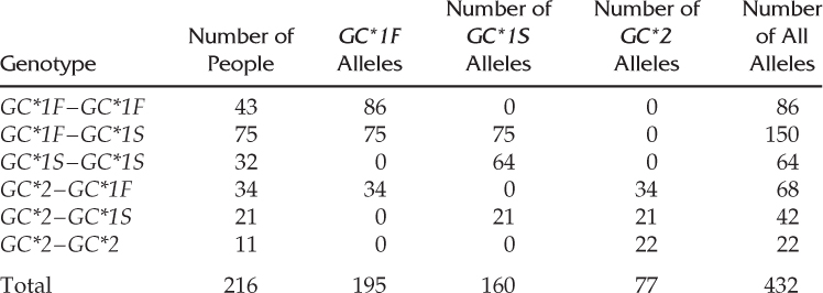
By summing up the columns, we see that there are 195 GC*1F alleles, 160 GC*1S alleles, and 77 GC*2 alleles for a total of 432 alleles.

Note that the sum of the three allele frequencies does not add up exactly to 1.0 (0.451 + 0.370 + 0.178 = 0.999). This is because of roundoff error; if you do all the computations of the allele frequencies to four decimal places, you will see that they do add up to 1.0 (0.4514 + 0.3704 + 0.1782 = 1.0).

2.1.2.3 An Alternative Method

The method used so far is often called the allele counting method because it relies on counting the number of different alleles over all genotypes. Another method of computing allele frequencies is based on the genotype frequencies. Returning to the first example used in this chapter, we have a locus with two alleles, A and a, in a hypothetical population of 150 people with the following genotypes: 54 AA, 72 Aa, and 24 aa. When we counted the alleles, we found 180 A alleles and 120 a alleles, giving allele frequencies of and .

Here is another way to calculate the allele frequencies. First, compute the genotype frequencies as before by dividing the number in each genotype by the total number of genotypes ( = 150). We did these calculations earlier in this chapter and obtained:

Note that I have assigned the symbol f to refer to genotype frequency and used subscripts to refer to the different genotypes. Thus fAA refers to the frequency of the AA genotype, fAa refers to the frequency of genotype Aa, and faa refers to the frequency of genotype aa. We can now compute the frequency of the A allele by adding the frequency of the AA genotype to half the frequency of the Aa genotype. Likewise, we can compute the frequency of the a allele by adding the frequency of half the Aa genotype to the frequency of the aa genotype. This is easier to express mathematically than in words (which is why we use symbols):

2.3

When we plug in the actual genotype frequencies in our example, we get the same allele frequencies as with the allele counting method:

Note that this method may not give the exact same results as the allele counting method if you did not compute the genotype frequencies using enough decimal places to avoid roundoff problems. My rationale for introducing this alternative method will be clear a little bit later.

Can you show why equation (2.3) works mathematically? The proof is shown in Appendix 2.1 at the end of this chapter.

2.2 What is Hardy–Weinberg Equilibrium?

2.4

These equations are often familiar to the introductory student in biological anthropology and biology classes. Following the initial math fear experienced by some students, just about everyone soon learns these simple equations. For example, if we know that p = 0.7 and q = 0.3 in the parental gene pool, we can quickly figure out the expected distribution of genotypes in the next generation as

The utility of predicting outcomes in the next generation can be illustrated with a more specific type of question. For example, let us imagine that the frequency of a harmful recessive allele is 0.01 and we want to know how many children will be born having two recessives, and hence a genetic disease. In this case, Hardy–Weinberg allows a quick answer: q2 = (0.01)2 = 0.0001, which is 1 in 10,000 offspring. Likewise, we could compute the expected proportion of heterozygotes that would not get the disease but would be carriers: 2pq = 2(0.99)(0.01) = 0.0198, which is 198 in 10,000 offspring.

Using the Hardy–Weinberg equations is straightforward. It is a second aspect of the Hardy–Weinberg law that causes more confusion. Both Hardy and Weinberg independently showed that, under certain conditions, the genotype and allele frequencies would remain constant from one generation to the next. In other words, Hardy–Weinberg equilibrium states that nothing changes (the very definition of equilibrium). Another way of saying that nothing changes is saying that there is no evolution! At this point in a typical lecture, everyone becomes rightfully perplexed. It is obvious from lab experiments, field studies, and the fossil record that organisms evolve all the time, which makes it difficult to understand why valuable lecture time (and textbook space) is being taken up by something that is clearly incorrect. The answer, which we then give in lecture, is that Hardy–Weinberg equilibrium gives us a baseline; we start with the case where nothing happens to show how something could happen! Although true, the underlying nature and utility of Hardy–Weinberg equilibrium often gets lost in the introductory course. Weiss and Kurland (2007:204) sum the confusing nature of Hardy–Weinberg equilibrium quite nicely, noting, “As one student griped, ‘Let me get this straight. When nothing happens … nothing changes? Duh.’”

I think that a major problem with understanding Hardy–Weinberg equilibrium is that it is difficult to reduce the concept and its implications into a simple but understandable definition. The idea instead takes more time and development, which is the goal of the remainder of this chapter.

2.3 The Mathematics of Hardy–Weinberg Equilibrium

Given allele frequencies p and q, equation (2.4) allows us to predict the expected genotype frequencies in the next generation. Where did equation (2.4) come from? There are several ways to answer this, and Hardy and Weinberg each used a somewhat different method to answer this question.

2.3.1 A Simple Proof

Here, I will start by demonstrating Hardy–Weinberg proportions [equation (2.4)] using a simple model of probability that uses an analogy for allele frequencies. Picture a cup filled with 100 small plastic beads, of which 60 are red and 40 are blue. We can say that the relative frequency of red beads is and the relative frequency of blue beads is . Imagine that all of these beads are mixed together and you pull one bead from the cup at random. What is the probability of getting a red bead? It is 0.6 (and the probability of getting a blue bead is 0.4). Now, imagine something a little more complicated. Pull out a bead, replace it in the cup, mix then beads together, and then pull out another bead. What is the probability of getting a red bead both times? We answer this using the and rule of probability from the previous chapter. The probability of getting two red beads is the probability of getting a red bead (0.6) multiplied by the probability of getting a red bead (0.6), which is 0.6 × 0.6 = 0.36. We can do the same type of computation to answer the question of repeating the same experiment and getting two blue beads. Here, the probability would be 0.4 × 0.4 = 0.16.

What about getting one red bead and one blue bead? This is a little more complicated because there are two ways of getting a red bead and a blue bead. The first way is to get a red bead on the first try and a blue bead on the second try, and the second way is the reverse—getting a blue bead on the first try and a red bead on the second try. We can solve this problem by breaking it down into several steps. First, what is the probability of getting a red bead on the first try and a blue bead on the second try? We use the and rule to figure this out and multiply the probability of getting a red bead (0.6) by the probability of getting a blue bead (0.4), which is 0.6 × 0.4 = 0.24. The second step is to determine the probability of the reverse happening, where we get a blue bead on the first try and a red bead on the second. Using the and rule, we get 0.4 × 0.6 = 0.24. Thus, we have a probability of 0.24 of getting a red bead followed by a blue bead, and we have a probability of 0.24 of getting a blue bead followed by a red bead. However, my initial question was only about the overall probability of getting one red bead and one blue bead, and the order does not matter. What is the probability of getting a red bead and then a blue bead or a blue bead and then a red bead? Here, we use the or rule and add the probabilities. The probability of getting one red bead and one blue bead, regardless of the order, is therefore 0.24 + 0.24 = 0.48.

We can now summarize the probability distribution of taking a bead from the cup at random, replacing it, and then taking a bead again at random:

Note that the sum of these probabilities is 1 (0.36 + 0.48 + 0.16), because we have listed all possible outcomes.

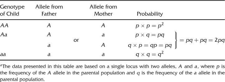
Going back to genetics, we can use the same principle. Instead of an experiment where we take a bead at random from a cup of beads, picture the process of reproduction of an allele that gets into the next generation as equivalent to taking an allele at random from a gene pool. Given two alleles, A and a, the possible genotypes in the next generation are AA, Aa, and aa. How do you get the AA genotype? The answer is when each parent contributes an A allele. To put this another way, what is the probability of a child getting an A allele from one parent and an A allele from the other parent? Given that p represents the frequency of the A allele, and is the probability of a given individual inheriting an A allele, the expected frequency for genotype AA in the next generation is p times p, = p2.

How about the genotype Aa? This can happen in one of two ways. The father can contribute an A allele and the mother can contribute an a allele, or the reverse can occur, where the father contributes an a allele and the mother contributes an A allele. The probability of the first situation occurring is p times q = pq. The probability of the second situation occurring is q times p = qp, which by the commutative law of algebra is the same as pq. Thus, the probability of getting an A allele from the father and an a allele from the mother or the reverse is pq + pq = 2pq.

The final genotype to consider is aa. The probability of obtaining this genotype is computed as the probability of both parents contributing an a allele, which is q times q = q2.

These proportions (AA = p2, Aa = 2pq, aa = q2) are the expected genotype frequencies [shown in equation (2.4)] expected under Hardy–Weinberg equilibrium. Table 2.1 summarizes the logic used here to demonstrate Hardy–Weinberg frequencies. Another method of deriving Hardy–Weinberg frequencies is to consider the genotypes for all possible offspring resulting from all possible random mating of parental genotypes (e.g., AA × AA, AA × Aa). This derivation can be found in most advanced population genetics texts (e.g., Hartl and Clark 2007).

Table 2.1 Using Simple Probability to Derive Hardy–Weinberg Proportionsa

Stay updated, free articles. Join our Telegram channel

Join