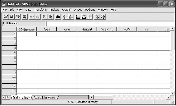
Notice that in the lower left corner, there’s one tab labeled Data View and another called Variable View (which is the screen we’re in now). Clicking on these allows you to switch between looking at the numbers themselves (the Data View) and the properties of the variables. It’s usually a good idea to start with the Variable View page, so you can name the variables and control what they look like on the screen. So, the first step is to give a name to each variable.
Defining the Variables
Name. There are a few rules for the variable names. They (1) must begin with a letter; (2) can be a mix of upper and lower case; (3) can contain the symbols @, #, _, and $; (4) cannot include a blank or any character not mentioned in (3), such as !, *, or ?; (5) cannot end with a period; and (6) cannot be more than 64 characters in length. You also have to avoid names that are used by SPSS for other purposes, such as LE (which means Less Than or Equal To), WITH, and a bunch of others. You don’t have to memorize these forbidden names; SPSS will tell you if you have blasphemed. Once you’ve filled in a name, SPSS fills in many of the other properties, but you can change these if you like, so let’s go through them.
Type. The are eight different “types” of variable. The default is Numeric, and this will suffice approximately 98.32% of the time. The only others you’re likely to use would be Date and String. As the name implies, date variables are for things like when the person was born or seen at the clinic. Once you click it, you’ll be offered a number of different ways of recording the date, such as dd.mmm.yy, mm/dd/yy, and eight other formats. One advantage of using date is that, given two dates, such as birth and visit, SPSS can use a function called YRMODA1 to calculate the exact age of the person at the time, saving you the agony and sparing the subject the necessity of lying.2 To most people, a string is something you use to tie up a package. But, for some strange reason, computer nerds use the term to describe a variable recorded as a word, such as “Male” or “Married.”
To change the type of variable, put the cursor anywhere inside the Type box and click once. The end of the box will become a grey square with three dots inside, and a new menu will appear, like the one below.
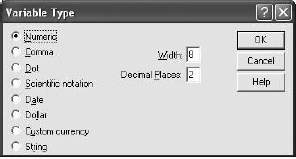
Width. Don’t worry about this unless the numbers you’ll be dealing with will have more than eight digits (the default).
Decimals. This controls how many decimal places are displayed in the Variable view; it doesn’t affect the storage of the data. So, if you have two decimal places (the default for numeric variables), and enter 5.249, it will appear on the screen as 5.25 but remain in memory as 5.249. We find the data easier to scan if you set it to zero for integers. As always, click anywhere inside the box, and use the arrows to modify the default. You can always change it later if you want to display more or fewer decimal places.
Label. Some variable names, such as Sex, ID Number, or Age, are sufficient to identify the contents. But, six months later, will you remember that ROMLKT3 refers to the range of motion of the left knee at time 3? Don’t count on it. With Label, you can give an extended description of the variable in something as close to English as you like; spaces and special characters are allowed.
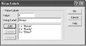
Values. This is used primarily for nominal and some ordinal variables. For example, if you’ve coded 1 = Never, 2 = Rarely, 3 = Often, and 4 = Always, you can use this option to both remind you of the coding scheme, and have the values printed out with the analyses. The default is None, but if you click inside the box, you’ll get a box that looks like:
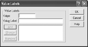
Enter 1 where it says Value (the u is underlined to indicate that you can also press Alt-u to get there), tab to the Value Label line and enter Never, and then click Add (or Alt-A). Continue to do this until all the values are entered and click on OK.
Missing. Do not forget this box if you have any missing values! Otherwise, you’ll end up with heights of 999 inches, or a lot of people who are 99 years old. Clicking inside this box brings up another dialog box:3
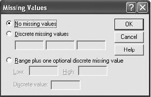
If you have anywhere from one to three different indicators for missing values, click the button next to Discrete missing values (or press Alt-d) and enter the numbers. If the numbers are sequential (e.g., 7 = Omitted, 8 = Refused to Answer, 9 = Other), you could check Range plus one optional discrete missing value. It’s also a good idea to go back to the Values box and enter 7 = Omitted, and so forth, so that the reasons for missingness get printed out.
Columns. This allows you to control how wide each column appears on the screen (Width affects the storage in memory, not the display). The default is, again, eight, and, yet again, can be changed by clicking anywhere in the box.
Align. This affects how the data are displayed. The default is right-justified for numbers and left-justified for string variables, but you can change these if you want to. Sometimes, when reading in a set of data, SPSS gets confused and interprets what should be a numeric variable as a string. If you reset the Type indicator, you may then want to change the justification to Right. We tend to avoid the Center option because (a) it should be spelled Centre, and (b) the decimal points don’t line up, making it more difficult to read the column.
Measure. The defaults are Scale for numeric variables and Nominal for string variables. The only other option is Ordinal. Some procedures differentiate among the types of measurements, so it’s a good idea to choose the right one. Change it in the usual way.
Entering the Data
If you now click on the tab in the lower left labeled Data View, the screen will change to reveal a spreadsheet, with the variables listed across the top, and where each line is for a new subject.
If you are entering data one subject at a time, hit after each value, and the cursor will automatically jump to the next variable. After the last, the cursor will move to the next subject. If you’re entering one variable at a time, then use after each value, and you’ll move from one subject to the next. And that’s all there is to it.
Saving Your Data
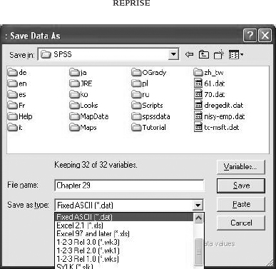
Click on File in the upper left hand corner, then Save As.… You can change the directory in which you save the file, then enter the name under which you want to keep the file. SPSS will automatically give the file the extension .sav. Later, if you click on a file with this extension, it will open SPSS with it as the active file. But, only some other statistical programs, such as SAS, will be able to read it. If you want the data saved in a format that other programs can use, then click on Save as type and select Fixed ASCII (*.dat) as the most flexible.
READING EXISTING FILES
In addition to .sav files, SPSS can read files created with spreadsheet programs, such as Excel, Lotus, and dBase; and some other statistical programs, such as SAS and Systat.4 If the file was created with a word processing program, it can be read as long as the file was saved with the extension .dat or .txt.
Reading .sav Files
You can open a data file created by SPSS by simply clicking on its name, or within SPSS itself. If SPSS is already running, then click File → Open → Data… and click on the filename.
Reading .txt or .dat Files
After you’ve gone through the File → Open → Data… routine, click the down arrow to the right of the Files of type: line and choose either Text (*.txt) or Data (*.dat), and then click on the filename. After you’ve done this, a “wizard” will open up,5 guiding you through the steps necessary to import the file.
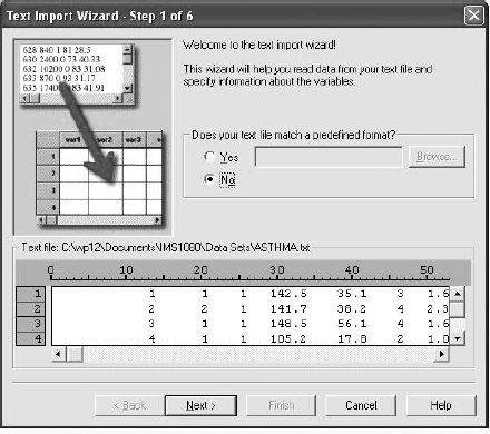
Your data most likely do not match a predefined format, so simply press Next and move on to Step 2.
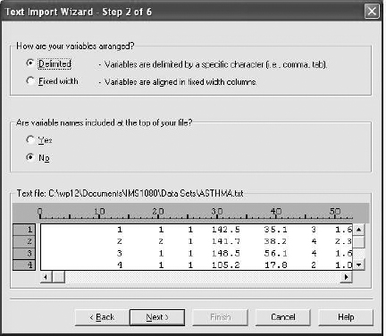
In most cases, the data are arranged in columns of fixed width, so change the default. Unless you entered variable names into the text file as the first row, leave that as the default. You’d possibly choose this option
if you had used a spreadsheet to enter the data, and assigned names to the variables.
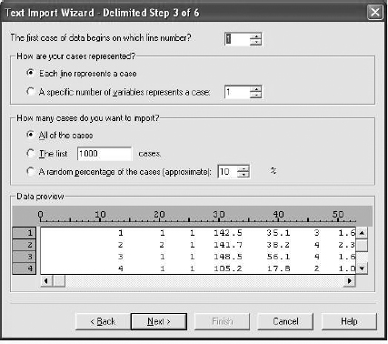
We can usually get through Step 3 by clicking Next and accepting all the options.
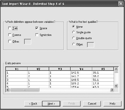
In Step 4, SPSS tries to differentiate among the variables by detecting where one ends and the next one starts. In most cases, it does a pretty good job. Otherwise, click on the vertical line and move it to the correct place. You can also delete variables at this stage; just read the instructions.

In Step 5, you can assign names to the variables and change their type (e.g., numeric, string, etc.). Alternatively, you can just click on Next > and do this in the Variable View page as we outlined previously. If you do this, the variables will be given default names of VI, V2, and so on.
Our experience has been that SPSS sometimes mistakes a numeric variable for a string, so watch out for that. If you wait for the Variable View to change it, you may also want to change the justification to right, because string variables are entered as left justified.
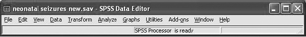
For the last page, ignore the options and just click Finish. The data will now be ready for you to (mis)apply everything you’ve been taught so far.
PLAYING WITH THE DATA
Once the data are in the machine, you can manipulate them in many ways—transform them, recode them, select only subjects who meet certain criteria, and on and on. We can’t show you everything,6 but we’ll tell you how to get started.
Transforming the Data
All of the commands we’ll discuss in this section are accessed through the pull-down menu called Transform on the top line (surprise, surprise).
REPRISE
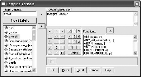
Compute. The Compute… command allows you to modify existing variables and to create new ones.When you call it up, you’ll get a screen like:
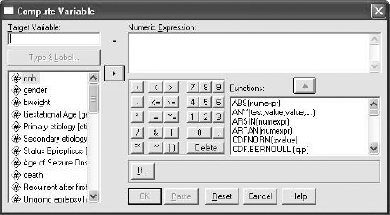
The first thing to do is to enter the name of the new variable you’ll be creating where it says Target Variable. What you do next depends on what you want to do. If, for example, you want to transform the variable using one of the functions (e.g., take the log to the base 10 or base e; take the square root; or calculate the number of times between two dates), select that function from the (very long) list, and press the button pointing upwards. What you’ll see is: with the cursor on the question mark. Then doubleclick the variable you want transformed, and you’ll have created a new variable; in this case, it would be the log of the original. If you’re not using one of the functions, then use the right arrow to move across the variable you’re operating on,7 and then use either the keypad on the screen or the keyboard to make the changes. For example, we recorded birthweight in grams. If you wanted to change it to ounces, you’d type in: and then hit OK. A new variable will magically appear in your data set.
Changing Only Some Subjects. So far, the transformations we’ve discussed affect all of the subjects. Sometimes, however, we want to change only selected cases. For example, we may have national norms for the birthweights of girls and boys, and want to express the weights as deviations from these national norms. Because the population means and standard deviations vary by gender, we have to do this separately for each group. For this, we use the button marked If…
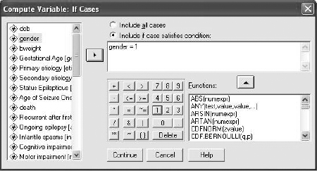
The default is Include all cases, so we first clicked on the button for Include if case satisfies condition, then brought over the variable we’re using as the basis of selection, entered the condition, and we’ll end by pressing Continue. This will bring us back to the previous screen, where we can enter the equation to create z-scores. We’ll then repeat the process, with gender = 2.
Recoding Variables. There are times when we may need to change how a variable is coded. One example is when we have a series of questions where 1 = Strongly Agree, 2 = Agree, 3 = Neutral, 4 = Disagree, and 5 = Strongly Disagree.8 But, sometimes, Strongly Agree may reflect endorsement of the trait we’re measuring; for other items, endorsement may be shown by answering Strongly Disagree. Before we do anything with the scale, such as factor analyzing it, we’d better be sure that 1 is reflecting strong endorsement for all items, or else our results will be meaningless.9 A different use of recoding is when we want to combine various categories of a nominal or interval variable. In the example we’re showing, we recorded nine different types of seizures that neonates may have had. However, when it came time to analyze the data, there were too few kids in each category for us to get any idea of what was going on, so it made sense to combine them into just four types. Here’s where the Recode command comes in.
When we pull down the Recode menu, we get two options: (1) to recode into the same variable, or (2) recode into a different variable. It’s almost always a good idea to choose the latter. This is especially true if you’re combining categories, because you can never go back and recapture the original data if you later change your mind and want to recode it differently. The first screen that comes up looks like:
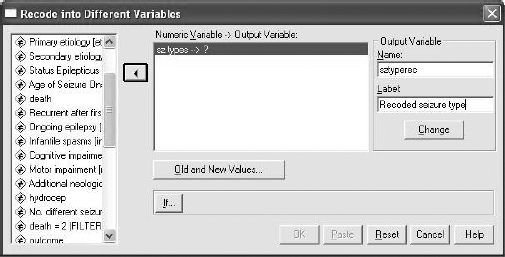
The variable sz.types is the name of the original variable. We entered a new name, sztyperec, in the box in the upper right corner, and gave it a label to remind ourselves that it’s the recoded variable. When we hit the Change button, the question mark in the middle box will be replaced with the new name. Then click on Old and New Values… to get the next screen.
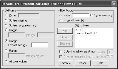
Here we’re about half way through the process. We began with Range: Lowest through and entered a 3 into the box; put a 1 in the box in the upper right corner called Value, and hit Add. In the second step, we clicked on Value in the upper left, entered a 4, and then a 2 in the box in the upper right, and hit Add again. At this stage, the values of 1, 2, and 3 in the original variable are combined into 1 in the new variable, and what was originally 4 is now coded as 2. We’ll continue doing this until all of the original nine values have been recoded, and then click on Continue.
There are many other things you can do, but this should be enough to get you started.
1 No, he was not a character in Star Wars. It stands for YeaR, MOnth, DAy.
2 Why is it that people will lie about their age, but never about their date of birth?
3 Why is it called a “dialog box “when it never answers you back? Shouldn’t it be a “monologue box”?
4 Because there’s a new version of SPSS every other year or so, this may change. You can check the types of files SPSS accepts after you’ve opened it, by clicking on Help → Topics, and then typing in open.
5 This terminology is probably a holdover from the days when computer programmers spent all of their time playing fantasy games.
6 Actually, we can, but we won’t. We have better things to do than copy the SPSS manuals. So, remember the computer nerds’ saying, “RTFM!,” which means “Read The Flippin’ Manual!”
7 In the mathematical, rather than surgical, sense.
8 For those who are interested, this is called a Likert scale. It’s also called a Likert scale for those who aren’t interested.
9 They may be meaningless even after recoding, but let’s not make things even worse for ourselves.
Stay updated, free articles. Join our Telegram channel

Full access? Get Clinical Tree


