. We can also use probability theory to make some general statements about the likelihood of a set of events occurring. For example, if we flip 10 coins, how many will come up heads? We might be very lucky and get 10 heads. We could also get 9 heads and 1 tail. The other possibilities are 8, 7, 6, 5, 4, 3, 2, 1, or 0 heads. Although we cannot tell beforehand what the specific outcome of any given toss of 10 coins will be, we can derive the probability of the occurrence of any of those outcomes. For example, the probability of getting all heads from 10 coin flips is roughly one in 1000 (0.000977), and the probability of getting 5 heads out of 10 coin flips is 0.246 (see any introductory statistics book for an explanation of how to do this).
Genetic drift is also a random process. Here, allele frequencies can fluctuate from generation to generation because of chance. Under Hardy–Weinberg equilibrium, we expect allele frequencies to remain constant from one generation to the next in the absence of mutation, selection, or gene flow. As noted in Chapter 2, an assumption of Hardy–Weinberg equilibrium is an infinite population size so there is no sampling deviation. In the real world, there are sampling deviations, and allele frequencies can increase or decrease by chance. As with coin flips, we cannot predict beforehand exactly what will happen as a result of genetic drift, but the principles of probability allow us to figure out the likelihood of different events occurring.
Although it is easy to give the definition of genetic drift as a random fluctuation in allele frequencies over time, it is more difficult to get a feel for what this actually means in an evolutionary context. We will start by considering the effect of sampling in a genetic context and then build to an example of genetic drift.
5.1.1 Genetic Sampling
Let us start with a simple example. Assume that there is a locus with two alleles, A and a, and that you have the heterozygous genotype Aa. When you have a child, you will pass along either the A allele or the a allele. Each event has a 50% chance of happening. Therefore, you might expect to pass on the A allele half of the time and the a allele half of the time. Now, suppose that you have four children. How many children do you expect to receive the A allele? Although your expectation would be to have two children with the A allele and two children with the a allele, in reality you could, by chance, have any of the following combinations:
- All four children will have the A allele (none will have the a allele).
- Three children will have the A allele and one child will have the a allele.
- Two children will have the A allele and two children will have the a allele.
- One child will have the A allele and three children will have the a allele.
- Zero children will have the A allele (they will all have the a allele).
Although we do not know beforehand which of these possibilities will occur, we can figure out the probability of any of these events happening. To start with, let us consider the case where all four children will receive the A allele. There is only one way for this to happen—the first child receives an A, the second child receives an A, the third child receives an A, and the fourth child receives an A. The probability that each child receives an A is  , which means that the probability that all will receive the A allele is the probability of the first receiving an A and the second receiving an A and the third receiving an A and the fourth receiving an A. Using the and rule from Chapter 1, we multiply the probabilities to get the probability that all four children receive the A allele as
We now move to the case where three children receive an A allele and one child receives an a allele. This is a little bit more complicated, because there are four different ways that this could occur: (1) the fourth child could receive the a, (2) the third child could receive the a, (3) the second child could receive the a, or (4) the first child could receive the a. Because the probability of receiving an a allele is the same as receiving an A allele  , the probability of any of these outcomes is
  . These four possibilities and their probabilities are:
To get the overall probability of getting some combination where three children receive the A allele and one child receives the a allele, we need to use the or rule from Chapter 1 and add the probabilities, which gives the total probability of getting 3 A alleles and 1 a allele as

We now move to the case where two children receive an A allele and two children receive an a allele. There are six different ways that can result in two A alleles and two a alleles:
Because each of these possibilities has a probability of  , the total probability of some any two children having an A allele is 6 × 0.0625 = 0.375.
The case where one child receives an A allele and three children receive an a allele is the same probability as the case where three children receives an A allele and one child receives an a allele. There are four ways for this to occur—Aaaa, aAaa, aaAa, and aaaA—each with a probability of 0.0625, giving a total probability of one A allele and three a alleles as 0.0625 × 4 = 0.25. Finally, the case where all four children receive an a allele (aaaa) is the same as the probability of all four children receiving an A allele, which is 0.0625. We now summarize the results in the following table:
| Number of A Alleles | Probability |
| 4 | 0.0625 |
| 3 | 0.2500 |
| 2 | 0.3750 |
| 1 | 0.2500 |
| 0 | 0.0625 |
Note that the total of all probabilities adds up to 1.0. Also, note that there is a lot of variation around the expected value of two A alleles. In fact, the majority of outcomes in this case will not have two A alleles (probability = 1 − 0.375 = 0.625 of having some number other than two A alleles). A difference from the expected outcome (two A alleles) is not unexpected if you think about it, because of the nature of probability. Think about a coin flipping analogy; if you flip four coins, you might get 4, 3, 2, 1, or 0 heads.
Deviations from expected values always result from sampling. The expected value for two A alleles out of four children is  , but this expected value will apply all the time only if we are talking about an infinite number of children! (Yes, this seems strange to consider in a biological sense, but it makes perfect sense mathematically.) In any real situation, we are sampling from an expected distribution of equal numbers of A and a alleles. If you have a finite and small number of children, then we will see different numbers of A alleles much of the time.
This sampling effect means that you may not pass on your genetic makeup exactly to your offspring. Now, consider this sampling effect happening in an entire population. The result is that the allele frequency among offspring may deviate from the allele frequency among the parents. This is genetic drift, or more precisely random genetic drift, because the process is random—sometimes an A allele is passed on, and sometimes an a allele is passed on.
5.1.2 A Simulation of Genetic Drift
In order to see how genetic drift works, we can perform a simple simulation experiment using a set of random numbers (Cavalli-Sforza and Bodmer 1971). For this experiment, we will start with our usual model of a locus with two alleles, A and a, where the initial allele frequencies are p = 0.5 and q = 0.5, respectively. Genetic drift will now be simulated for a population of five people. Because each person has two alleles, this means, that we are dealing with 10 alleles. Given a probability of 0.5 for any allele being an A allele, how many A alleles will we get if we sample 10 alleles? This is analogous to flipping 10 coins to see how many come up heads. Here, however, we are dealing with the probability that an allele present in the parental generation will be passed on to the offspring generation. The expected value (given an initial allele frequency of 0.5) is 5 in 10 A alleles. We know, however, that sampling could result in any number from 0 to 10 A alleles.
Most often, we use computer programs to simulate the process of genetic drift, which essentially involves a measure of “coin flipping” inside the computer. Here, we will use a different method of simulation by employing a random-number table. Such tables consist of randomly chosen digits (from 0 to 9) and are useful in demonstrating random processes. Here, I used the table of random digits from Rohlf and Sokal (1995), which is a table of 10,000 random digits produced by a computer program. I randomly selected a starting point in the table and wrote out the first 10 digits listed from left to right:

We now use these numbers by setting up a rule that matches these digits with the probability of selecting an A or an a allele. Because the initial frequency for A is 0.5, we will use half of the digits (0–4) to represent the A allele and the other half of the digits (5–9) to represent the a allele. An easy way to do this is to note which of the 10 digits represents the A allele by setting those digits (0, 1, 2, 3, or 4) in boldface. This gives us

Because 6 of 10 digits are in the range from 0 to 4, this gives us a new allele frequency in the offspring generation of  . The allele frequency has changed from 0.5 to 0.6 in a single generation because of genetic drift.
I continued the simulation to the next generation by drawing the next set of 10 random digits from the table:

Because the allele frequency in the parental generation is now 0.6, we have to adjust the coding scheme accordingly, letting the digits 0–5 represent the A allele (which is because the range of these 6 of 10 possible digits corresponds to the new probability of 0.6). We now indicate the digits corresponding to the A alleles in boldface, giving

There are now five A alleles out of 10, giving a new allele frequency of  .
.
I then extended the analysis to the next generation by picking the next 10-digit string of numbers:

Because the parental allele frequency is again p = 0.5, we let the digits 0–4 represent the A allele. Setting these in boldface gives

There are 4 out of 10 alleles that are A alleles, giving an allele frequency of p = 0.4. In this case, the allele frequency did not change from one generation to the next.
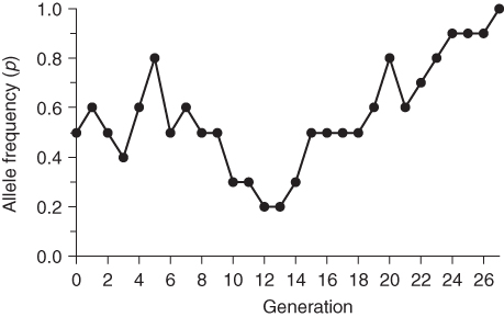
I continued the simulation using additional random digits over a number of generations. The results are graphed in Figure 5.1. Note that the allele frequency fluctuates over time—sometimes it increases, sometimes it decreases, and sometimes it stays the same. Note that the simulation ends in generation 27 when the allele frequency drifts up from 0.9 to 1.0. Because there are only A alleles in the population, there will be no further change in allele frequency—it will remain at 1.0 unless the a allele is reintroduced through mutation or migration.
Figure 5.1 Computer simulation of genetic drift. This simulation is based on a population size of 5 individuals (10 alleles) and starts with an allele frequency of p = 0.5. Random genetic drift is simulated using a table of random numbers as described in the text. Note that the simulation ends at generation 27 when the allele frequency has drifted down to zero. No further change is possible because there are only A alleles in the population. Fixation or extinction of an allele is the eventual outcome of genetic drift.
5.1.3 The Outcome of Genetic Drift
It is important to remember that each time you simulate genetic drift you will see some differences. If I were to start the above simulation at a different starting point in the table of random numbers, the run would look different. We can see the random nature of genetic drift by comparing several simulations that all start with the same initial allele frequency and population size. Here, and throughout the remainder of the chapter, the simulations are based on a computer program written to simulate genetic drift. The logic of the program is the same as the simulation above, but the computer is used to generate the random numbers and tally the number of A alleles in each generation (which is much faster!).
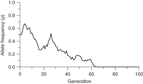
In order to illustrate the random nature of genetic drift, I performed 100 simulations of drift over 100 generations, each starting with an initial allele frequency of p = 0.5 for a population of N = 50 individuals (we will continue using the symbol N to indicate population size throughout this text). I selected 3 of the 100 runs were selected to show different outcomes for genetic drift; these are shown in Figures 5.2, 5.3, 5.4. Figure 5.2 shows a case where the allele frequency fluctuates both up and down, and after 100 generations is essentially back to the point where it started. Figure 5.3 also shows fluctuation over time, but eventually drifts up to a frequency of p = 1.0 after 78 generations. When the allele frequency reaches this value, it has reached a state of fixation; there will be no further change because all of the alleles in the population are A alleles. The only way there could be any more change would be if there were a mutation or if another allele were introduced from another population (gene flow). Figure 5.4 shows a similar outcome, where, after some fluctuation over time, the allele frequency eventually drifts down to a value of p = 0 after 64 generations. Here, the A allele has reached a state of extinction in that all of the A alleles are gone. No further change will take place unless there is an A allele introduced through mutation or migration.
Figure 5.2 Computer simulation of genetic drift in a population of N = 50 individuals, run 1. The initial allele frequency is p = 0.5. The large amount of random fluctuation of allele frequency over time is characteristic of genetic drift in a small population. Compare this graph with two other runs using the same starting parameters as in Figures 5.3 and 5.4.
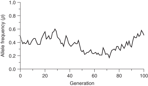
Figure 5.3 Computer simulation of genetic drift in a population of N = 50 individuals, run 1. The initial allele frequency is p = 0.5. The large amount of random fluctuation of allele frequency over time is characteristic of genetic drift in a small population. Note that there is no further change in allele frequency after generation 78, at which point the allele has become fixed in the population. Compare this graph with two other runs using the same starting parameters as in Figures 5.2 and 5.4.
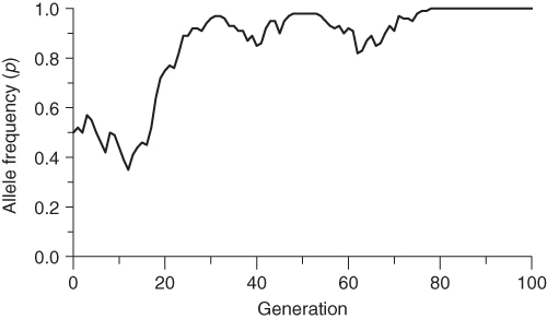
Figure 5.4 Computer simulation of genetic drift in a population of N = 50 individuals, run 1. The initial allele frequency is p = 0.5. The large amount of random fluctuation of allele frequency over time is characteristic of genetic drift in a small population. Note that there is no further change in allele frequency after generation 64, at which point the allele has become extinct in the population. Compare this graph with two other runs using the same starting parameters as in Figures 5.2 and 5.3.
The above examples are meant only to give the reader a taste of some extreme outcomes. In reality, any value between p = 0 and p = 1 is possible. This brings up an interesting question—although we cannot predict the outcome of any specific case of genetic drift, can we make any predictions about what outcomes are more likely? Yes, such predictions can be made using advanced probability theory. Another (and easier to visualize) way of seeing general trends in genetic drift is to use computer simulation of drift over a large number of runs in order to get a visualization of the range of outcomes. Such an example is shown in Figure 5.5, which simulates 100 generations of drift in a population of 50 reproductive adults. Note that the population size here refers only to the number of individuals that are actually reproducing in any given generation (hence the term reproductive adults). The distinction between different measures of population size is discussed in more detail later in this chapter; for the moment, it is only necessary to remember that we are counting only those individuals who are reproducing. In addition, we are assuming that the population size stays the same each generation; in other words, 50 adults have 50 offspring that survive to become the adults in the next generation, who then have 50 offspring, and so forth. Again, we will deal with problems with this assumption later, but for now, we will concentrate only on the overall impact of genetic drift.
Figure 5.5 Computer simulation of genetic drift showing the results of 100 runs of 100 generations of drift in a population of N = 50 reproductive adults starting with an initial allele frequency of p = 0.5 for each run. Note the tendency for genetic drift to cause the allele frequency to become extinct (p = 0) or fixed (p = 1) than to have intermediate values. Given enough time, genetic drift will always result in extinction or fixation.
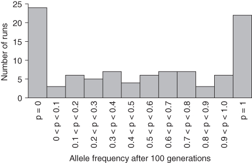
Because each simulation run is different, we need to conduct a fairly large number of runs to get an idea of average trends. For Figure 5.5, I had the computer program run the analysis from scratch 100 times in order to generate a distribution of outcomes of drift. What should be immediately clear from Figure 5.5 is that many of the runs led to extinction (p = 0), similar to what you saw in Figure 5.4, or fixation (p = 1), similar to what you saw in Figure 5.3. The rest of the allele frequencies are more or less evenly distributed between the extreme values of p = 0 and p = 1.
So many of the runs resulted in allele extinction or fixation because genetic drift tends toward extremes over time. In fact, probability theory shows that, given enough time, genetic drift will always lead to extinction or fixation. The distribution of allele frequencies after 100 generations shown in Figure 5.5 is well on the way toward the expected end result of all runs showing extinction or fixation.
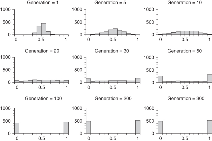
The distribution of allele frequencies changes over time. An example is shown in Figure 5.6, which is based on 1000 simulations of genetic drift in a population of N = 20 reproductive adults. Each simulation starts with an initial allele frequency of p = 0.5. Figure 5.6 shows the allele frequency distribution at different points in time for the first 300 generations of genetic drift. The first graph (upper left of the figure) shows the allele frequency distribution after a single generation of genetic drift. The allele frequencies all cluster close to the mean (and expected) allele frequency of 0.5, although some runs drifted as low as p = 0.3 or as high as p = 0.775. By 5 generations, drift has led to a greater spreading of allele frequencies, which increases further by 10 generations. By 20 generations, the distribution is fairly flat, and by 50 generations there is a tendency for the majority of runs to have resulted in either extinction (p = 0.0) or fixation (p = 1.0). This U-shaped distribution is even more apparent by generation 100 and generation 200, where only a small number of runs resulted in values other than p = 0.0 or p = 1.0. By 300 generations, all of the runs have resulted in either extinction of fixation. According to probability theory, if we ran this simulation an infinite number of times (or at least a very large number of times), half of the runs will result in extinction and half in fixation. The actual numbers in Figure 5.6 are 484 runs that resulted in extinction and 516 runs that resulted in extinction, which is indistinguishable statistically from the expected 50 : 50 ratio.
Figure 5.6 Computer simulation of genetic drift showing the results of 1000 runs of genetic drift for different numbers of generations in a population of N = 20 reproductive adults starting with an initial allele frequency of p = 0.5 for each run. The categories for the histograms are those used in Figure 5.5; categories are for 0.1 increment between p > 0.0 and p < 1.0, with separate categories for p = 0.0 (extinction) and p = 1.0 (fixation), shown on the left and right sides of the horizontal axis (abscissa). The vertical axis (ordinate) measures the number of runs.
In the above example, we expected that half of the runs would result in extinction and half would result in fixation. The reason for this number (50 : 50) is that the initial allele frequency was 0.5; that is, half the alleles were A alleles and half were a alleles. Another way to envision this is to consider a starting point of p = 0.5 from which drift will sometimes move to the left of this mean (<0.5) and sometimes will move to the right (>0.5). Each generation, drift will continue to move left or right in a random fashion until the allele becomes extinct (p = 0.0) or fixed (p = 1.0). Because we started at p = 0.5, the distance to randomly drift down to p = 0.0 is equal to the distance to randomly drift up to p = 1.0. Thus, we expect (subject to sampling error) an equal number of cases where extinction and fixation occur.
Given enough time, the ultimate fate of drift is either extinction or fixation, but the relative number of times that each occurs depends on the initial starting value of p. For example, what would we expect if we repeated the same experiment of drift (1000 runs of drift over 300 generations based on a population of N = 20 reproductive adults) but started each run with an initial allele frequency of p = 0.2? Because drift is a random process, we expect that allele frequencies will drift below p = 0.2 and above p = 0.2, just as they did when we started with p = 0.5. In this case, however, the distance to extinction (moving from p = 0.2 to p = 0.0) is much less than the distance to fixation (where the allele frequency would have to move from p = 0.2 to p = 1.0). Thus, even though we would eventually see all possible runs result in either extinction or fixation, we also expect extinction to occur much more often because the initial starting value in this case (p = 0.2) is closer to extinction than fixation.
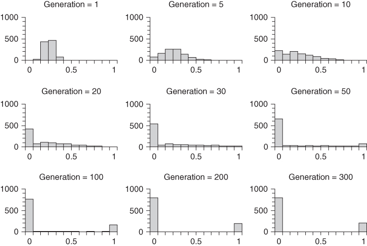
These expectations can be tested using computer simulation. Figure 5.7 shows the results of 1000 runs of genetic drift over 300 generations in a population of N = 20 reproductive adults where each run starts at an initial allele frequency of p = 0.2. As with our earlier example, Figure 5.7 shows the distribution of allele frequencies after different numbers of generations have passed. Note that over time the allele frequency initially flattens out and then becomes a distribution that has an increasing number of cases ending in allele extinction or fixation. This is what also happened in Figure 5.6, but now there are many more cases of extinction than fixation. After 300 generations have passed, all of the runs have resulted in either extinction or fixation. Unlike the scenario in Figure 5.6, where the number of extinctions and fixations was roughly equal, now there are many more extinctions. Specifically, after 300 generations, we see in Figure 5.7 that 801 runs resulted in extinction and 199 runs resulted in fixation.
Figure 5.7 Computer simulation of genetic drift showing the results of 1000 runs of genetic drift for different numbers of generations in a population of N = 20 reproductive adults starting with an initial allele frequency of p = 0.2 for each run. The categories for the histograms are those used in Figure 5.5; categories are for 0.1 increment between p > 0.0 and p < 1.0, with separate categories for p = 0.0 (extinction) and p = 1.0 (fixation), shown on the left and right sides of the horizontal axis. The vertical axis measures the number of runs.
The major difference between the simulations shown in Figures 5.6 and 5.7 is that there are fewer cases of fixation in the second set of simulations. The only parameter that was different about these two simulations is the initial allele frequency. In the first set of simulations (Figure 5.6), the initial allele frequency was p = 0.5. The relative frequency of fixation in this simulation was 516 runs out of 1000 total runs, giving a rate of  . In the second set of simulations (Figure 5.7), the initial allele frequency was p = 0.2 and the relative frequency of fixation was 199 out of 1000 runs, giving a rate of
  . You may note that in both cases the observed frequency of fixation was almost identical to the initial allele frequency (0.516 vs. 0.5 and 0.199 vs. 0.2). This is not a coincidence, but an expected outcome. In terms of probability theory, the probability of fixation of an allele is equal to the initial frequency of the allele. The small, and statistically insignificant, differences between the simulation experiments and the theoretical expectations are due to sampling error. The expected probability of allele fixation is based on an idealized mathematical model with an infinite number of runs. In the real world, there will be some deviations because we are looking at a smaller number of cases.
As will be described in detail below, the amount of genetic drift is dependent on population size. The above simulation experiments used very small population sizes (N = 20) in order to show a lot of drift over the course of 300 generations. If we used a larger population size, it would likely take much longer than 300 generations to reach a state where each run resulted in allele extinction or fixation. In general, the larger the population size, the longer this will take on average (Kimura and Ohta 1969). In a mathematical sense, any finite population will eventually drift to extinction or fixation. However, in a real-world setting, it could easily take a very large (and unrealistic) number of generations to do so.
5.2 Genetic Drift and Population Size
In all the above simulations of drift, we needed to consider the number of reproductive adults in the population. The number of breeding individuals in a population determines the extent of likely genetic drift. In short, drift is likely to be greater in a single generation in a small population than in a larger population. The smaller the population, the more likely drift will lead to a larger change in allele frequency. For example, a change in allele frequency in one generation from 0.5 to 0.6 is much more likely for a population of 50 reproductive adults than a population of 500 reproductive adults.
Before considering the impact of population size on drift, it is important to consider exactly what we mean by population size. In the context of demography, the size of a population is the total number of people alive at any given point in time. In terms of genetic drift, however, we must only consider those individuals who are actually contributing genetically to the next generation—that is, the number of reproductive adults. We consider the entire population as being made up of three nonoverlapping generations: a prereproductive generation, a reproductive generation, and a postreproductive generation. Individuals that have already reproduced belong to the last generation, and individuals who have not yet reached reproductive age (children) belong to the next generation. If we want to think about the potential for drift in any given generation, we have to focus on the current number of reproductive adults.
Sometimes we contrast these two different views of population size by labeling them census population size and breeding population size. The former refers to everyone in the population, whereas the latter refers to only the reproductive adults. This is an important distinction, because if we want to consider the amount of drift possible in a village of, say, 100 people, we have to remember that the actual breeding population size is much less than 100 after we exclude the younger (prereproductive) and older (postreproductive) individuals. One commonly used rule of thumb is to take breeding population size as one-third of census population size, based on the assumption that a population can be divided into three broad age groups—prereproductive, reproductive, and postreproductive (Cavalli-Sforza and Bodmer 1971).
Although useful for rough comparisons, this measure can be a bit crude as the proportion of individuals of reproductive age in any given population can vary depending on the age structure of the population. For example, among the Dobe !Kung, a hunter–gatherer society of the Kalahari Desert in southern Africa, the number of individuals of reproductive age (15–49 years) in 1968 was 282, out of a total census size of 569, which is almost half (Howell 2000). It is also important to consider cultural influences on age at reproduction. Among the !Kung, women often start reproducing early in their lives—the average age of a mother at the birth of her first child is 19 (Howell 2000). In other cultures, age at first reproduction may be later. In nineteenth–twentieth-century Ireland, for example, it was common for a number of men and women to marry late or to remain single and not reproduce because of a complex interplay of social and economic factors (Kennedy 1973). In addition, as will be described later, many other factors further influence the degree of genetic drift seen in relation to population size. For the moment, we will consider a simple model where we can clearly identify the exact number of reproductive adults in the population (we are also making some other implicit assumptions that will become clear later in this chapter).
5.2.1 How Does Population Size Affect Genetic Drift?
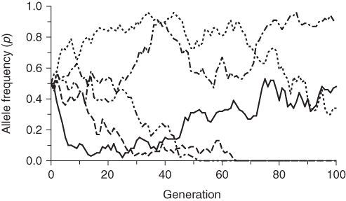
The easiest way to see how population size affects genetic drift is to compare a number of runs for different values of population size. Figures 5.8, 5.9, 5.10 do just that. Each of these figures shows the results of five independent runs of genetic drift (to get an idea of the range of likely outcomes) for 100 generations, all starting from an initial allele frequency of p = 0.5. The difference between the three figures is the population size used in the simulations. Figure 5.8 uses a population size of N = 50, Figure 5.9 uses a population size of N = 500, and Figure 5.10 uses a population size of N = 5,000.
Figure 5.8 Five computer simulations of genetic drift for population size of N = 50 and an initial allele frequency of p = 0.5. The five runs are indicated by different types of lines. Note the wide range of fluctuation in allele frequency. Compare this graph with Figure 5.9 (population size N = 500) and Figure 5.10 (population size N = 5000).
Stay updated, free articles. Join our Telegram channel

Full access? Get Clinical Tree


