8.1 The Evolutionary Impact of Gene Flow
One assumption of Hardy–Weinberg equilibrium is that the population remains closed to other populations; that is, there is no gene flow. In fact, throughout our discussions of mutation, drift, and selection, we have always focused on a single population. In the real world, however, the existence of a single-population species is very rare. For example, humans live in thousands of populations around the world, which are all interconnected by varying levels of gene flow in the present and the past. What is the evolutionary impact of gene flow?
8.1.1 Introducing New Alleles
Thus far, the only way that we have seen a new allele enter a population is through mutation; drift and selection can increase or decrease the frequency of a new mutation, but they cannot bring about a new allele. Although mutation is the ultimate source of all new alleles, a new mutant allele can be introduced into a different population through gene flow. Picture two populations, A and B, where everyone has two copies of a specific allele. Now, imagine a mutation occurring in population A. Although it is possible for the same mutation to occur in population B, it is highly unlikely to happen in the same generation. On the other hand, if someone from population A carries the mutant allele and moves to population B and reproduces, the mutant allele is now established in population B through gene flow. Gene flow allows the spread of new mutants throughout a species, subject in each population to the further effects of drift and selection (we can see how complex microevolution can get when considering all four evolutionary forces at the same time).
8.1.2 Reducing Genetic Differences between Populations
The main impact of gene flow is to reduce genetic differences between populations. Here, we can picture gene flow as analogous to mixing paint. Imagine starting with two gallon cans of paint, one with red paint and one with white paint. Take a cup of paint from the red can and mix it into the white can at the same time as taking a cup of white paint and mixing it into the red can. After mixing, the can of red paint is slightly lighter and the can of white paint is slightly pinker. If you repeat the mixing, the color of the paint in the two cans will become increasingly similar. After enough cups of paint have been swapped and mixed, you will have two identical cans of pink paint.
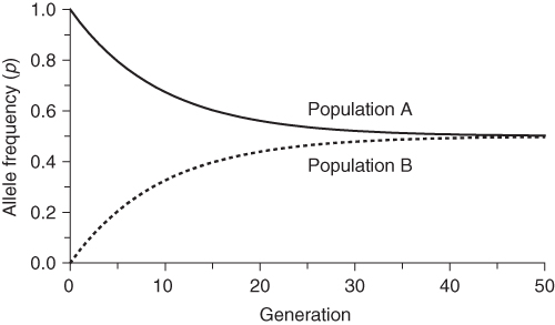
We can picture gene flow in an analogous manner where the alleles of two or more populations are mixed together. Although alleles are not paint, and do not actually merge together, the point here is that the mixing of gene pools can alter the allele frequencies. As an example, imagine two populations (A and B), where the frequency of a given allele is p = 1.0 in population A and p = 0.0 in population B. Now, imagine that 5% of the individuals in population A move into population B and reproduce there, while 5% of the individuals in population B move into population A and reproduce there. In other words, the two populations exchange 5% of their genes. This means that 95% of the individuals in population A remain in population A. The allele frequency in population A a generation later is made up of the mixing of 95% from population A with an allele frequency of p = 1.0 and 5% from population B with an allele frequency of p = 0.0. This gives the new allele frequency in population A of

At the same time, we can figure out the allele frequency in population B a generation later by noting that it will consist of 5% from population A with an allele frequency of p = 1.0 and 95% from population B with an allele frequency of p = 0.0, giving

Because of gene flow, the allele frequencies in populations A and B have changed from 1.0 and 0.0 to 0.95 and 0.05. They are still quite different, but closer than they were initially. Over time, gene flow will make the two populations increasingly similar. To figure out the allele frequencies in the next generation, we use the same mixing proportions (95% and 5%) and use the new allele frequencies for populations A and B (p = 0.95 and p = 0.05). Thus, the allele frequency in population A after two generations of gene flow is

and the allele frequency in population B is

If we go to the third generation, we simply use these new allele frequencies with the same amount of mixing to get allele frequencies of

for population A, and

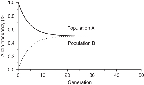
for population B. We can repeat the same process many times from one generation to the next to see the long-term effect of gene flow. Figure 8.1 shows the results of gene flow for 50 generations. We see that gene flow quickly reduces the difference between the two populations such that they are almost identical after 40 generations.
Figure 8.1 Simulation of gene flow between two populations. Populations A and B start with allele frequencies of p = 1.0 and q = 0.0, respectively. With each generation, 5% of each population is exchanged with the other, leading to a reduction of the allele frequency differences over time.
Now that we have seen the basic effect of gene flow to reduce genetic differences between populations, we can examine several different models of gene flow in more specific detail. As with previous treatment of evolutionary forces, we will consider gene flow by itself to start with and then add complexity by examining the interaction with other evolutionary forces.
8.2.1 The Island Model
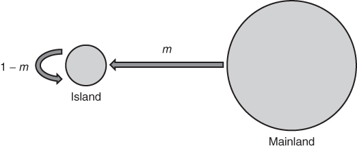
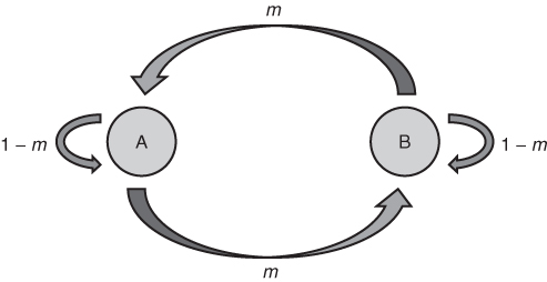
The simplest place to start with understanding how gene flow works is to examine the case of one-way migration as shown in the island model (or more specifically, the continent–island model, as there are other types of island models used in population genetics). Here, we imagine an island that receives a certain amount of migration from the mainland, but this migration is strictly in one direction—no migration occurs from the island to the mainland. In this way, we can see what effect gene flow from the mainland has on the allele frequencies of the island. We use the symbol m to illustrate the migration rate, which is the proportion of alleles in the island that come from the mainland each generation. Because m represents the genetic contribution from the mainland, this means that the proportion (1 − m) of the island’s alleles comes from the island (because the two proportions, one from the mainland and one from the island, have to add up to 1). The dynamics of this model are shown in Figure 8.2.
Figure 8.2 The island model. Gene flow is one-way from a large mainland population into a smaller island, such that the allele frequency in the mainland affects the allele frequency in the island, but not the other way around. m represents the migration rate each generation and is the proportion of alleles in the island’s next generation that comes from the mainland. The quantity (1 − m) represents the proportion of alleles in the island’s next generation that comes from the island. For example, a value of m = 0.1 indicates that 10% of the alleles in the island come from the mainland, and (1 − m) = 0.9 indicates that 90% of the alleles on the island come from the island in the previous generation.
In order to simulate the one-way gene flow under the island model, we need to know the initial allele frequencies of the island and the mainland. Here, we use p0 to represent the initial allele frequency (in generation 0) of the island. We use the symbol P (uppercase p) to represent the allele frequency of the mainland. Because our model only involves gene flow, and since there is no gene flow from the island to the mainland, this means that the mainland allele frequency P stays the same from one generation to the next. In order to calculate the allele frequency on the island in the next generation, we multiply the proportions of alleles from the island and the mainland by their allele frequencies, respectively. For the first generation, this will be
where m is the migration rate (i.e., the proportion of alleles from the mainland). Because P (and hence mP) does not change, we can also predict the allele frequency on the island after an additional generation of one-way gene flow by substituting p1 for p0 in the above equation, giving
Because this is an iterative equation of the type encountered in Chapter 4, we can use the method in Appendix 4.1 to derive the allele frequency in any given generation, pt as
(see Appendix 8.1 for the derivation).
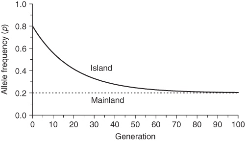
The effect of one-way gene flow in the island model is shown in Figure 8.3 using an initial allele frequency for the island of p0 = 0.8, a constant allele frequency on the mainland of P = 0.2, and a per generation migration rate of m = 0.05. Over time, the allele frequency on the island becomes increasingly similar to that on the mainland, showing that the genetic makeup of the island is eventually replaced by that of the mainland.
Figure 8.3 Change in allele frequencies over time in the island model. The allele frequencies in each generation are computed using equation (8.1). The initial allele frequency on the island is p0 = 0.8. The allele frequency on the mainland, which is constant over time, is P = 0.2. The amount of one-way gene flow per generation (the migration rate) is m = 0.05. Over time, the island will become increasingly similar to the mainland.
8.2.2 Two-Way Gene Flow
The island model focuses on gene flow in one direction, and allele frequency does not change in the source population (mainland). Although this model fits some cases, a model that allows gene flow in two directions is more applicable to many situations. Figure 8.4 shows a simple model of two-way gene flow where the rate of migration is the same in both directions. Here, two populations, A and B, exchange migrants and genes at a rate of m per generation. This number represents the proportion of alleles in one population from the other population. Each population receives a proportion (1 − m) of its alleles from itself.
Figure 8.4 Two-way gene flow. Two populations, A and B, each have a proportion m of alleles from the other population and a proportion (1 − m) of alleles from themselves.
We start with the rate of gene flow per generation m and allele frequencies for population A and B in generation t, which we label as  and
and  (the first subscript refers to the population and the second subscript, to the generation). We can estimate the allele frequency in population A in the next generation (t + 1) by multiplying the allele frequencies of each population by the proportion of alleles provided to population A:
Likewise, the allele frequency in population B in the next generation is derived using the same logic, such that
As an example, consider initial allele frequencies of  and
and  and a gene flow rate of m = 0.1 per generation. After one generation of gene flow, the allele frequency is population A is computed using equation (8.2), giving

and the allele frequency in population B is computed using equation (8.3), giving

Note that the allele frequencies in the two populations are closer than before. We can then extend gene flow to subsequent generations by taking these new allele frequencies and substituting them back into equations (8.2) and (8.3), giving allele frequencies in the second generation of

and

This process can be extended to additional generations as shown in Figure 8.5, which shows how the allele frequencies become increasingly similar to each other. In fact, by about 20 generations, the allele frequencies are essentially the same. Note that the curves resemble those seen in Figure 8.1, which was also modeled using two-way gene flow. When you compare Figures 8.1 and 8.5, you will see that convergence of the allele frequencies is faster in Figure 8.5. This is because the rate of gene flow used to construct Figure 8.5 (m = 0.1) is greater than that used in Figure 8.1 (m = 0.05).
Figure 8.5 Two-way gene flow with initial allele frequencies of pA = 1.0 and pB = 0.0 and a rate of gene flow of m = 0.1. Compare the speed at which the allele frequencies converge with that of Figure 8.1, where a lower rate of gene flow (m = 0.05) was used.
8.2.3 Kin-Structured Migration
The examples using two-way gene flow show clearly that gene flow acts to make populations more similar to each other over time, and that the higher the rate of gene flow, the more rapidly this convergence occurs. Gene flow is most often considered a homogenizing force that reduces the genetic difference between populations. However, this is technically correct only if we make the hitherto unstated assumption that the individuals that migrate and reproduce are a random sample of the source population. This may not always be the case. In some situations, the migrants may be related. One way that migrants can be related occurs in some small-scale human societies when part of a population splits off and then fuses with another population. There are other examples of entire families moving into a new population. When the migrants are related, we call this kin-structured migration.
Anthropologist Alan Fix has looked at the genetic effects of kin-structured migration on genetic differences between populations (Fix 1978, 1999). Gene flow usually acts to reduce differences between populations, and kin-structured migration can slow this process down, or even reverse it in some cases, leading to increased genetic differences between groups. Fix (1978) looked at kin-structured migration among the Semai Senoi, a swidden (slash-and-burn) agricultural group in the Malayan Peninsula in Malaysia. Over time, populations split and the resulting groups of migrants were (and are still) typically kin. Using simulations incorporating genetic drift and gene flow based on the demography of the population, Fix found that although kin-structured migration flow would still reduce genetic differences between Semai Senoi populations over time, the actual reduction would be less than if the migrants were simply a random sample. Although kin-structured migration is not universal, it has been found in other human populations, including the Yanomama Indians of South America as well as the founding populations of Tristan da Cunha and Plymouth in the United States (Fix 1999).
8.3 Gene Flow and Genetic Drift
Of course, gene flow does not operate alone, and to get a better idea of the genetic effects of gene flow, we need to consider how it interacts with genetic drift. To do this, we need to consider in more detail the concept of between-group variation introduced in the first chapter. In previous chapters, we have considered the effect of microevolution on genetic variation (measured by heterozygosity or a similar statistic) within a single population. This within-group variation refers to genetic differences (variation) between individuals within a single population. Between-group variation (also referred to as among-group variation) looks at differences between the genetic compositions of two or more populations. For example, if two populations each have allele frequencies of p = 0.6 and q = 0.4, there is no genetic difference between these populations, although there is variation within both populations.
On average, genetic drift increases genetic differences between populations. The ultimate fate of genetic drift is the fixation or extinction of an allele. Because this is a random process, over time different alleles will become fixed in different populations, thus increasing the genetic variation between populations. On the other hand, gene flow counters drift and reduces genetic differences between populations. Clearly, the two evolutionary forces act in opposition to each other, and we need to see how and when they might reach an equilibrium between the amount of between-group variation added by genetic drift and the amount lost by gene flow.
8.3.1 Measuring Genetic Variation between Populations
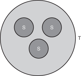
Before looking at the equilibrium between genetic drift and gene flow, we need to consider briefly how we can measure between-group variation. In Chapter 5, when we considered the balance between mutation and genetic drift, we looked at heterozygosity (H) as a measure of the amount of genetic variation within a population. Here, we consider another measure (FST) as a measure of genetic variation between populations. Picture a region made up of a number of populations. Examples include a group of villages on a Pacific island, a group of rural towns in the English countryside, or a group of different ethnic neighborhoods in a city, among many other possible examples. Although we will consider real examples from human populations later in this chapter, for the moment we will approach this idea in a more abstract manner by considering a number of subpopulations that make up the total population. Figure 8.6 shows a graphic illustration where the total population (T) is made up of three subpopulations (S). This type of model refers to a hierarchical population structure where the subpopulations are nested inside the total population.
Figure 8.6 Hierarchical population structure. The total population (T) is made up of three subpopulations (S).
For our purpose here, we can look at genetic variation in three different ways:
1. The amount of genetic variation in the total population
2. The amount of genetic variation within the subpopulations
3. The amount of genetic variation between the subpopulations
Note that quantities 2 and 3 make up the total amount of variation:

When we look at the effects of gene flow and drift (or other factors) on genetic differences between groups, we are interested in what proportion of the total variation is due to genetic variation. This proportion, denoted FST, is
Because total variation is made up of the sum of within-group variation and between-group variation, we can express the above equation in terms of total and within-group variation as
This measure looks at variation in the subpopulations (S) relative to the total (T) population.
A simple example will help clarify these concepts. Imagine a single locus with two alleles, A and a, with the following allele frequencies in three subpopulations that have equal population sizes:
Subpopulation 1: p = 0.6, q = 0.4
Subpopulation 2: p = 0.52, q = 0.48
Subpopulation 3: p = 0.5, q = 0.5
We also need to know the allele frequencies in the total population, pooling all three subpopulations into a single group. Because the three populations all have equal population sizes, we can simply take the average allele frequencies, designated as p and q , as
If the subpopulations had different population sizes, then we would have computed an average weighted by population size.
The first thing we are interested in looking at is the amount of genetic variation within the total population. This quantity is the heterozygosity based on the allele frequencies of the total population (p and q ), and is computed as shown in Chapter 5 for two alleles as

Note that we use the subscript ‘T’ to designate that this refers to the total population. The next quantity of interest is the amount of genetic variation within the subpopulations. Here, we simply take the heterozygosity for each subpopulation and then average them. Using the formula for heterozygosity for two alleles (H = 2pq), we obtain heterozygosity values of H = 0.48 for subpopulation 1, H = 0.4992 for subpopulation 2, and H = 0.5 for subpopulation 3. The average of these three values gives us an amount of genetic variation within groups of
Here, we use the subscript W to designate variation within subpopulations.
We now return to equation (8.4) and see that we have measures for both total variation (HT) and within-group variation (HW), and can derive FST as
For our simple example, HT = 0.4968 and HW = 0.4931, giving an FST value of 0.0074. As this is a proportion, we can state that 0.74% of the total genetic variation is due to variation between groups, leaving 99.26% of the total genetic variation due to variation within groups.
The FST values in human populations frequently range from close to zero to higher values between 0.05 and 0.10 (within 5–10%) (Jorde 1980). As will be outlined in more detail below, genetic drift increases FST and gene flow decreases FST. A population with a moderate FST is often characterized by relatively small populations and/or low rates of gene flow. Large populations and/or high rates of gene flow tend to produce smaller FST values.
8.3.2 Equilibrium between Gene Flow and Genetic Drift
You might be wondering where the symbol F in FST comes from. We have seen other examples of F earlier in the book, including the concept of identity by descent under inbreeding (Chapter 3) and the probability of identity by descent due to genetic drift (Chapter 5). The use of the same letter is not accidental; all of these uses refer to various types of a fixation index, which is a measure of the proportional reduction in heterozygosity relative to Hardy–Weinberg conditions. Equation (8.5) shows the proportional reduction that occurs when a population is structured into subpopulations (S) rather than consisting of one large population (T) within which all individuals have an equal chance of mating. Whenever a population is subdivided in this way, there will be some reduction in heterozygosity, and FST provides an index of the degree of reduction.
Because we are dealing with the probability of identity by descent, we can extend models developed earlier to the case of an interaction of gene flow and genetic drift. Like mutation, gene flow acts to reduce the probability of identity by descent—an allele introduced from outside a population means that there will be no common ancestry within the population. When looking at gene flow, we define m as the rate of gene flow per generation, which is interpreted as the probability that an allele comes from outside the population. In practical terms, we typically estimate m in human populations as the proportion of individuals in a population that were born in another population. Identity by descent is possible only when both alleles have not come into the population due to gene flow. In Chapter 5, we dealt with a similar idea when considering the interaction between mutation and drift, which means that the logic and derivation of the probability of identity by descent under gene flow and drift can be derived by substituting the rate of gene flow (m) for the rate of mutation (μ) in Appendix 5.8. Thus, equation A5.6 becomes
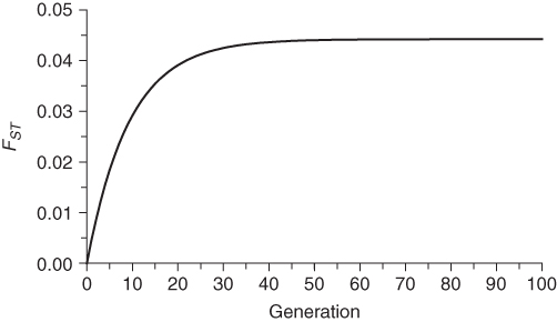
Figure 8.7 shows values of FST over time for a population size of N = 100 and a migration rate of m = 0.05. FST increases rapidly at first because of the cumulative effects of genetic drift. Over time, gene flow moderates this increase, until an equilibrium of between-group variation is reached. As before, N as used here refers to the breeding population size in an idealized model, and in actual analysis we would want to consider the effective population size.
Figure 8.7 Change in FST over time for N = 100 and m = 0.05. The FST values were computed using equation (8.6) starting with an initial value of FST = 0. Initially FST increases rapidly as a result of genetic drift, but then levels off because of gene flow to approach an equilibrium of roughly FST = 0.044.
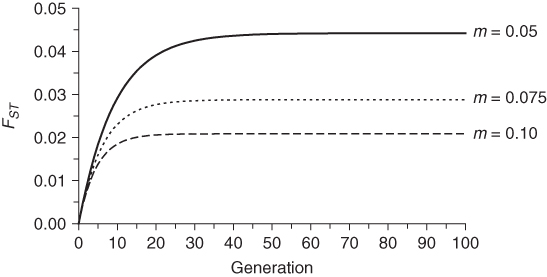
The eventual equilibrium between genetic drift and gene flow depends on both population size and migration rate. Figure 8.8 shows three examples of changes in FST over time where the population size is held constant at N = 100 but the migration rate varies. The higher the migration rate, the lower the equilibrium value of FST. Figure 8.9 shows three examples of change in FST over time where the migration rate is held constant at m = 0.05 but the population size varies. The larger the population size, the smaller the equilibrium value of FST.
Figure 8.8 Change in FST over time for different values of migration rate. In each case, the population size was set to N = 100. The FST values were computed using equation (8.6) starting with an initial value of FST = 0. The larger the migration rate, the smaller the equilibrium value of FST.
Stay updated, free articles. Join our Telegram channel

Full access? Get Clinical Tree


