A Incidence (Incident Cases)

Incidence is the frequency of occurrences of disease, injury, or death—that is, the number of transitions from well to ill, from uninjured to injured, or from alive to dead—in the study population during the time period of the study. The term incidence is sometimes used incorrectly to mean incidence rate (defined in a later section). Therefore, to avoid confusion, it may be better to use the term incident cases, rather than incidence. Figure 2-1 shows the annual number of incident cases of acquired immunodeficiency syndrome (AIDS) by year of report for the United States from 1981 to 1992, using the definition of AIDS in use at that time.

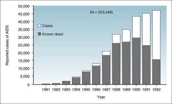
Figure 2-1 Incident cases of acquired immunodeficiency syndrome in United States, by year of report, 1981-1992.
The full height of a bar represents the number of incident cases of AIDS in a given year. The darkened portion of a bar represents the number of patients in whom AIDS was diagnosed in a given year, but who were known to be dead by the end of 1992. The clear portion represents the number of patients who had AIDS diagnosed in a given year and were still living at the end of 1992. Statistics include cases from Guam, Puerto Rico, the U.S. Pacific Islands, and the U.S. Virgin Islands.

(From Centers for Disease Control and Prevention: Summary of notifiable diseases—United States, 1992. MMWR 41:55, 1993.)

B Prevalence (Prevalent Cases)

Prevalence (sometimes called point prevalence) is the number of persons in a defined population who have a specified disease or condition at a given point in time, usually the time when a survey is conducted. The term prevalence is sometimes used incorrectly to mean prevalence rate (defined in a later section). Therefore, to avoid confusion, the awkward term prevalent cases is usually preferable to prevalence.

C Illustration of Morbidity Concepts

The concepts of incidence (incident cases), point prevalence (prevalent cases), and period prevalence are illustrated in Figure 2-2, based on a method devised in 1957.¹ Figure 2-2 provides data concerning eight persons who have a given disease in a defined population in which there is no emigration or immigration. Each person is assigned a case number (case no. 1 through case no. 8). A line begins when a person becomes ill and ends when that person either recovers or dies. The symbol t₁ signifies the beginning of the study period (e.g., a calendar year) and t₂ signifies the end.

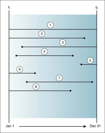
Figure 2-2 Illustration of several concepts in morbidity.
Lines indicate when eight persons became ill (start of a line) and when they recovered or died (end of a line) between the beginning of a year (t₁) and the end of the same year (± t₂). Each person is assigned a case number, which is circled in this figure. Point prevalence: t₁ = 4 and t₂ = 3; period prevalence = 8.

(Based on Dorn HF: A classification system for morbidity concepts. Public Health Rep 72:1043–1048, 1957.)

In case no. 1, the patient was already ill when the year began and was still alive and ill when it ended. In case nos. 2, 6, and 8, the patients were already ill when the year began, but recovered or died during the year. In case nos. 3 and 5, the patients became ill during the year and were still alive and ill when the year ended. In case nos. 4 and 7, the patients became ill during the year and either recovered or died during the year. On the basis of Figure 2-2, the following calculations can be made. There were four incident cases during the year (case nos. 3, 4, 5, and 7). The point prevalence at t₁ was four (the prevalent cases were nos. 1, 2, 6, and 8). The point prevalence at t₂ was three (case nos. 1, 3, and 5). The period prevalence is equal to the point prevalence at t₁ plus the incidence between t₁ and t₂, or in this example, 4 + 4 = 8. Although a person can be an incident case only once, he or she could be considered a prevalent case at many points in time, including the beginning and end of the study period (as with case no. 1).

D Relationship between Incidence and Prevalence

Figure 2-1 provides data from the U.S. Centers for Disease Control and Prevention (CDC) to illustrate the complex relationship between incidence and prevalence. It uses the example of AIDS in the United States from 1981, when it was first recognized, through 1992, after which the definition of AIDS underwent a major change. Because AIDS is a clinical syndrome, the present discussion addresses the prevalence of AIDS, rather than the prevalence of its causal agent, human immunodeficiency virus (HIV) infection.

In Figure 2-1, the full height of each year’s bar shows the total number of new AIDS cases reported to the CDC for that year. The darkened part of each bar shows the number of people in whom AIDS was diagnosed in that year, and who were known to be dead by December 31, 1992. The clear space in each bar represents the number of people in whom AIDS was diagnosed in that year, and who presumably were still alive on December 31, 1992. The sum of the clear areas represents the prevalent cases of AIDS as of the last day of 1992. Of the people in whom AIDS was diagnosed between 1990 and 1992 and who had had the condition for a relatively short time, a fairly high proportion were still alive at the cutoff date. Their survival resulted from the recency of their infection and from improved treatment. However, almost all people in whom AIDS was diagnosed during the first 6 years of the epidemic had died by that date.

The total number of cases of an epidemic disease reported over time is its cumulative incidence. According to the CDC, the cumulative incidence of AIDS in the United States through December 31, 1991, was 206,392, and the number known to have died was 133,232.² At the close of 1991, there were 73,160 prevalent cases of AIDS (206,392 − 133,232). If these people with AIDS died in subsequent years, they would be removed from the category of prevalent cases.

On January 1, 1993, the CDC made a major change in the criteria for defining AIDS. A backlog of patients whose disease manifestations met the new criteria was included in the counts for the first time in 1993, and this resulted in a sudden, huge spike in the number of reported AIDS cases (Fig. 2-3). Because of this change in criteria and reporting, the more recent AIDS data are not as satisfactory as the older data for illustrating the relationship between incidence and prevalence. Nevertheless, Figure 2-3 provides a vivid illustration of the importance of a consistent definition of a disease in making accurate comparisons of trends in rates over time.

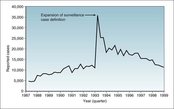
Figure 2-3 Incident cases of AIDS in United States, by quarter of report, 1987-1999.
Statistics include cases from Guam, Puerto Rico, the U.S. Pacific Islands, and the U.S. Virgin Islands. On January 1, 1993, the CDC changed the criteria for defining AIDS. The expansion of the surveillance case definition resulted in a huge spike in the number of reported cases.

(From Centers for Disease Control and Prevention: Summary of notifiable diseases—United States, 1998. MMWR 47:20, 1999.)

Prevalence is the result of many factors: the periodic (annual) number of new cases; the immigration and emigration of persons with the disease; and the average duration of the disease, which is defined as the time from its onset until death or healing. The following is an approximate general formula for prevalence that cannot be used for detailed scientific estimation, but that is conceptually important for understanding and predicting the burden of disease on a society or population:

In the specific case of AIDS, its incidence in the United States is declining, whereas the duration of life for people with AIDS is increasing as a result of antiviral agents and other methods of treatment and prophylaxis. These methods have increased the length of survival proportionately more than the decline in incidence, so that prevalent cases of AIDS continue to increase in the United States. This increase in prevalence has led to an increase in the burden of patient care in terms of demand on the health care system and dollar cost to society.

A similar situation exists with regard to cardiovascular disease. Its age-specific incidence has been declining in the United States in recent decades, but its prevalence has not. As advances in technology and pharmacotherapy forestall death, people live longer with disease.

A Definition

In epidemiology, risk is defined as the proportion of persons who are unaffected at the beginning of a study period, but who experience a risk event during the study period. The risk event may be death, disease, or injury, and the people at risk for the event at the beginning of the study period constitute a cohort. If an investigator follows everyone in a cohort for several years, the denominator for the risk of an event does not change (unless people are lost to follow-up). In a cohort, the denominator for a 5-year risk of death or disease is the same as for a 1-year risk, because in both situations the denominator is the number of persons counted at the beginning of the study.

Care is needed when applying actual risk estimates (which are derived from populations) to individuals. If death, disease, or injury occurs in an individual, the person’s risk is 100%. As an example, the best way to approach patients’ questions regarding the risk related to surgery is probably not to give them a number (e.g., “Your chances of survival are 99%”). They might then worry whether they would be in the 1% group or the 99% group. Rather, it is better to put the risk of surgery in the context of the many other risks they may take frequently, such as the risks involved in a long automobile trip.

B Limitations of the Concept of Risk

Often it is difficult to be sure of the correct denominator for a measure of risk. Who is truly at risk? Only women are at risk for becoming pregnant, but even this statement must be modified, because for practical purposes, only women aged 15 to 44 years are likely to become pregnant. Even in this group, some proportion is not at risk because they use birth control, do not engage in heterosexual relations, have had a hysterectomy, or are sterile for other reasons.

Ideally, for risk related to infectious disease, only the susceptible population—that is, people without antibody protection—would be counted in the denominator. However, antibody levels are usually unknown. As a practical compromise, the denominator usually consists of either the total population of an area or the people in an age group who probably lack antibodies.

Expressing the risk of death from an infectious disease, although seemingly simple, is quite complex. This is because such a risk is the product of many different proportions, as can be seen in Figure 2-4. Numerous subsets of the population must be considered. People who die of an infectious disease are a subset of people who are ill from the disease, who are a subset of the people who are infected by the disease agent, who are a subset of the people who are exposed to the infection, who are a subset of the people who are susceptible to the infection, who are a subset of the total population.

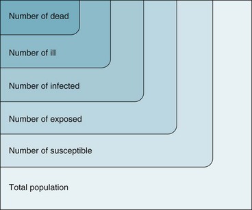
Figure 2-4 Graphic representation of why the death rate from an infectious disease is the product of many proportions.
The formula may be viewed as follows:

If each of the five fractions to the right of the equal sign were 0.5, the persons who were dead would represent 50% of those who were ill, 25% of those who were infected, 12.5% of those who were exposed, 6.25% of those who were susceptible, and 3.125% of the total population.

The proportion of clinically ill persons who die is the case fatality ratio; the higher this ratio, the more virulent the infection. The proportion of infected persons who are clinically ill is often called the pathogenicity of the organism. The proportion of exposed persons who become infected is sometimes called the infectiousness of the organism, but infectiousness is also influenced by the conditions of exposure. A full understanding of the epidemiology of an infectious disease would require knowledge of all the ratios shown in Figure 2-4. Analogous characterizations may be applied to noninfectious disease.

The concept of risk has other limitations, which can be understood through the following thought experiment. Assume that three different populations of the same size and age distribution (e.g., three nursing homes with no new patients during the study period) have the same overall risk of death (e.g., 10%) in the same year (e.g., from January 1 to December 31 in year X). Despite their similarity in risk, the deaths in the three populations may occur in very different patterns over time. Suppose that population A suffered a serious influenza epidemic in January (the beginning of the study year), and that most of those who died that year did so in the first month of the year. Suppose that the influenza epidemic did not hit population B until December (the end of the study year), so that most of the deaths in that population occurred during the last month of the year. Finally, suppose that population C did not experience the epidemic, and that its deaths occurred (as usual) evenly throughout the year. The 1-year risk of death (10%) would be the same in all three populations, but the force of mortality would not be the same. The force of mortality would be greatest in population A, least in population B, and intermediate in population C. Because the measure of risk cannot distinguish between these three patterns in the timing of deaths, a more precise measure—the rate—may be used instead.

A Definition

A rate is the number of events that occur in a defined time period, divided by the average number of people at risk for the event during the period under study. Because the population at the middle of the period can usually be considered a good estimate of the average number of people at risk during that period, the midperiod population is often used as the denominator of a rate. The formal structure of a rate is described in the following equation:

Risks and rates usually have values less than 1 unless the event of interest can occur repeatedly, as with colds or asthma attacks. However, decimal fractions are awkward to think about and discuss, especially if we try to imagine fractions of a death (e.g., “one one-thousandth of a death per year”). Rates are usually multiplied by a constant multiplier—100, 1000, 10,000, or 100,000—to make the numerator larger than 1 and thus easier to discuss (e.g., “one death per thousand people per year”). When a constant multiplier is used, the numerator and the denominator are multiplied by the same number, so the value of the ratio is not changed.

The crude death rate illustrates why a constant multiplier is used. In 2011, this rate for the United States was estimated as 0.00838 per year. However, most people find it easier to multiply this fraction by 1000 and express it as 8.38 deaths per 1000 individuals in the population per year. The general form for calculating the rate in this case is as follows:

Rates can be thought of in the same way as the velocity of a car. It is possible to talk about average rates or average velocity for a period of time. The average velocity is obtained by dividing the miles traveled (e.g., 55) by the time required (e.g., 1 hour), in which case the car averaged 55 miles per hour. This does not mean that the car was traveling at exactly 55 miles per hour for every instant during that hour. In a similar manner, the average rate of an event (e.g., death) is equal to the total number of events for a defined time (e.g., 1 year) divided by the average population exposed to that event (e.g., 12 deaths per 1000 persons per year).

A rate, as with a velocity, also can be understood as describing reality at an instant in time, in which case the death rate can be expressed as an instantaneous death rate or hazard rate. Because death is a discrete event rather than a continuous function, however, instantaneous rates cannot actually be measured; they can only be estimated. (Note that the rates discussed in this book are average rates unless otherwise stated.)

B Relationship between Risk and Rate

In an example presented in section II.B, populations A, B, and C were similar in size, and each had a 10% overall risk of death in the same year, but their patterns of death differed greatly. Figure 2-5 shows the three different patterns and illustrates how, in this example, the concept of rate is superior to the concept of risk in showing differences in the force of mortality.

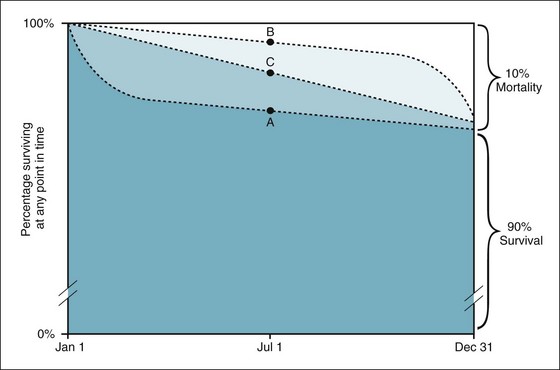
Figure 2-5 Circumstances under which the concept of rate is superior to the concept of risk.
Assume that populations A, B, and C are three different populations of the same size; that 10% of each population died in a given year; and that most of the deaths in population A occurred early in the year, most of the deaths in population B occurred late in the year, and the deaths in population C were evenly distributed throughout the year. In all three populations, the risk of death would be the same—10%—even though the patterns of death differed greatly. The rate of death, which is calculated using the midyear population as the denominator, would be the highest in population A, the lowest in population B, and intermediate in population C, reflecting the relative magnitude of the force of mortality in the three populations.

Because most of the deaths in population A occurred before July 1, the midyear population of this cohort would be the smallest of the three, and the resulting death rate would be the highest (because the denominator is the smallest and the numerator is the same size for all three populations). In contrast, because most of the deaths in population B occurred at the end of the year, the midyear population of this cohort would be the largest of the three, and the death rate would be the lowest. For population C, both the number of deaths before July 1 and the death rate would be intermediate between those of A and B. Although the 1-year risk for these three populations did not show differences in the force of mortality, cohort-specific rates did so by reflecting more accurately the timing of the deaths in the three populations. This quantitative result agrees with the graph and with intuition, because if we assume that the quality of life was reasonably good, most people would prefer to be in population B. More days of life are lived by those in population B during the year, because of the lower force of mortality.

Rates are often used to estimate risk. A rate is a good approximation of risk if the:

Stay updated, free articles. Join our Telegram channel

Join