Digital Analysis of Cells and Tissues
Peter H. Bartels
Deborah Thompson
Leopold G. Koss
Digital microscopy provides a numeric representation of diagnostic imagery that offers some distinct advantages over conventional visual microscopy. Digital data establish a permanent reproducible record that can readily be distributed, archived, communicated and displayed at variable magnifications. They are ideally suited for teleconsultation and, as virtual slides, for teaching. The numeric representation also provides the basis for quantitative analysis of diagnostic images. Quantification introduces a wealth of novel information and concepts.
How does all of this relate to established diagnostic practice? Knowledge in diagnostic cyto- and histopathology is communicated in linguistic terms and concepts. Although these terms are fuzzy, they theoretically carry an extraordinary amount of highly specific information. Quantification of diagnostic images is not meant to replace visual images or create new diagnostic concepts. Rather, the challenge is to express well-proven diagnostic clues and concepts in numeric terms. It has become clear, however, that quantification generates a body of “digital knowledge” that is uniquely derived from computer processing of digitally represented images in cytopathology and histopathology. Developments in information science have allowed an objective, quantitative evaluation of these images, which can be expressed in understandable linguistic terms and are based on an accumulation of multiple diagnostic clues. These methods have led to the development of automated or semiautomated diagnostic decision support systems, and to objective standards for diagnosis defined by digital imagery. Table 46-1 lists the principal targets of applications of image analysis techniques. Many, but not all, of these targets are discussed in this chapter which is dedicated to the description of the methods and their principal applications based on simple instrumentation.
THE DIGITIZED IMAGE
The microscopic image is formed as a distribution of brightness and darkness in an “image plane.” It is a continuous distribution. In video-photometry, this image is projected onto the faceplate of a video camera, typically a charge-coupled device (CCD) array. The CCD samples the image by its array of sensor elements and the image is now represented
by an array of discrete points or picture elements called pixels.
by an array of discrete points or picture elements called pixels.
TABLE 46-1 TARGETS OF DIGITAL IMAGE ANALYSIS OF CELLS AND TISSUES | ||||||||||||||||||||||||||||||||||||
|---|---|---|---|---|---|---|---|---|---|---|---|---|---|---|---|---|---|---|---|---|---|---|---|---|---|---|---|---|---|---|---|---|---|---|---|---|
| ||||||||||||||||||||||||||||||||||||
The light energy sensed at each point is recorded in digital form and stored in computer memory.
It is essential to project the microscopic image onto the CCD at an adequate magnification. The finest detail that the original image can offer is restricted by features of the objective, such as the numerical aperture. The magnification at the faceplate of the CCD should be chosen to maintain “useful magnification,” i.e., to preserve the objective’s resolving power by the CCD elements. In practice, one would oversample, i.e., have two or more CCD elements covering an image region corresponding to the point spread function of the objective.
Figure 46-1A shows a digitized image of a human embryonic lung cell, recorded in 1966 at the University of Chicago in the study that initiated the taxonomic intracellular analysis system (TICAS) project (Wied et al, 1968). The numbers are “pixel optical density values.” Today’s digitized images are sampled at a spacing approximately 40 × closer, yielding several thousand pixels per nucleus (Fig. 46-1B). Images are recorded in the form of “light intensity values,” ranging from 0 to 255, with 0 denoting total darkness and 255 full 100% transmission. It is customary to convert the light intensity value image to pixel optical density (OD) values. These range from optical density OD = 0, denoting full brightness, to OD = 3.00, indicating a light transmission of 1 per 1,000, i.e., very dark. In practice, one multiplies these values by 100 in order to store them in memory as integer form. A pixel OD of 0.15 would be stored as 15.
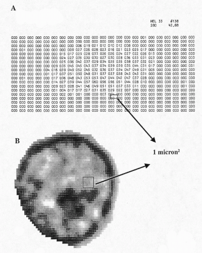 Figure 46-1 A. The digitized image of human embryonic lung cell, recorded at 1 micron resolution. The numbers are “pixel optical density” values. B. An image of a hematoxylin-stained nucleus, recorded at 6 pixels per micron, and enlarged to show the pixelation. |
Visual Versus Computed Image Information
Much of the information that can be derived from digitized imagery does not have a visual counterpart and provides novel information of potential diagnostic value. The difference between visual and computed image information is best demonstrated by a familiar example. Figure 46-2 shows a sample of printed text. A reader recognizes letters, words, and even the language: all of this is visual information. However, if asked “what is the relative frequency of occurrence
of the vowel ‘o’ compared to that of the vowel ‘e’?”, no immediate answer can be given. Yet, these relative frequencies characterize the text and provide an objective, computed descriptive feature. One could ask how often is the letter “k” followed by the letter “l,” or how often do two consonants follow each other? The pixel optical density values in a digitized image offer exactly the same kind of computed descriptive features in their 2-dimensional spatial and statistical distribution.
of the vowel ‘o’ compared to that of the vowel ‘e’?”, no immediate answer can be given. Yet, these relative frequencies characterize the text and provide an objective, computed descriptive feature. One could ask how often is the letter “k” followed by the letter “l,” or how often do two consonants follow each other? The pixel optical density values in a digitized image offer exactly the same kind of computed descriptive features in their 2-dimensional spatial and statistical distribution.
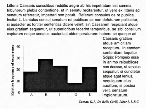 Figure 46-2 Demonstration of visual and digital information: written text and computed frequency distribution of its vowels. |
The potential of digital diagnostic pathology and cytology, though, far exceeds the mere statistical/descriptive representation of diagnostic evidence. Through power of variance-analytic procedures, the numeric representation allows the detection of subtle but consistently expressed differences between and among similar targets. Computational procedures allow the detection of diagnostic evidence that is not readily perceived by visual examination. Distinctive changes in the chromatin patterns of nuclei of benign cells in the presence of premalignant or malignant lesions are one example (Wied et al, 1980; Sherman and Koss, 1983; Bibbo et al, 1986; Montag et al, 1989; Bibbo et al, 1990; Palcic et al, 1994; MacAulay et al, 1995; Susnik et al, 1995; Bartels et al, 1998). Computer processing here truly expanded our ability to provide diagnostic information.
In the visual assessment of a malignant tumor, the information offered by the image is transformed by a pathologist into a “grade.” The equivalent in machine vision is direct mapping of a microscopic image to a numerically defined point on a continuous progression curve that may offer additional information beyond grade.
Quantification of diagnostic images requires accurate and precise data acquisition. Image processing is then applied to the acquired data to extract diagnostic information, followed by numeric/analytic evaluation and diagnostic interpretation. In practice, one may distinguish between the digital assessment of cell images or nuclei, i.e., cytometry and karyometry, and the assessment of histopathologic sections, i.e., histometry. Of these, karyometry has proven to be particularly informative.
It is useful to distinguish three steps in the analysis of data: image processing, image analysis, and image interpretation.
In image processing, an algorithm that may be useful in subsequent extraction of diagnostic information is applied to the image. For example, a pixel optical density value threshold may be established, or a contrast-enhancing processing algorithm may be applied to define the targets of the study. In image processing, the input and the output are both represented by images.
In image analysis, specific diagnostic information is extracted from the image. Here, the first step is usually scene segmentation to delineate objects of interest; for example, the outline of a nucleus. While the input in image analysis is an image, the output is a set of “features”—numeric values which characterize the sample and which contain diagnostic information.
In image interpretation, the measures obtained from image analysis are evaluated by a mathematic/analytic process in order to assign a diagnostic label; for example, a cell may be classified as either normal or abnormal. The diagnostic label may also be a grade or a numeric value of a progression index established for a lesion or set of lesions.
Quantification of diagnostic image assessment involves methodologies derived from a wide range of scientific disciplines. It is the objective of this chapter to present an introduction to these methodologies and their theoretical bases and to illustrate each with practical examples.
SCENE SEGMENTATION
Procedures and Strategies
Scene segmentation is a crucial first step in quantitative image analysis (Abele et al, 1977; Weszka, 1978; Brenner et al, 1981; Juetting et al, 1983; Abmayr et al, 1987; Bartels and Thompson, 1994; Thompson et al, 1995). Any error in the delineation of objects propagates to the values used to define diagnostic features. For example, incorrect outline of a nuclear boundary is the principal cause for “false alarms” in automated screening for cervical cancer.
The problems with scene segmentation depend on the target. Under ideal circumstances, the microscopic image is based on a monolayer of single cells against a clean background, free of debris. At the other extreme, scene segmentation has to deal with complex imagery such as is seen in histologic sections of glands.
There are two distinctly different approaches to scene segmentation. The first is image-oriented. Here, the image in its entirety is processed by a segmentation algorithm. All objects in the scene are segmented by the same procedure.
The second approach is object-oriented. First, a search for “objects” is conducted, usually by applying an image processing algorithm, such as threshold-setting to the image. Then, each recognized object is outlined by a chaincode (see below) and stored (Freeman, 1961). Next, each of the stored objects is categorized and processed by a suitable segmentation algorithm. The object-oriented approach thus employs a flexible strategy, where different objects in the scene may be segmented by different procedures.
The image-oriented approach has the advantage of simplicity and speed. However, the selected algorithm may work well on some targets but fail with others. The object-oriented approach has a much higher software requirement and may be somewhat slower, but can better handle complex imagery. The result in both approaches is an outline of objects of interest, usually represented as a chaincode.
A chaincode is a list of values that begins with an x,y image coordinate for the first or start-pixel in the display, followed by a set of directions to the next pixel, etc. until the code returns to the start-pixel. One may define “the next pixel” depending on the system used. The definition is important because the approach to the pixelation of a small object may affect features such as perimeter length, object roundness, and object area (Bartels and Thompson, 1994; Neal et al, 1998).
Many segmentation algorithms are available. There are algorithms strictly based on the optical density of the object or pixel optical density thresholding. These may be used interactively by an observer who may adjust the threshold
up and down until an object’s outline agrees with the visual boundary. However, a fixed threshold may interfere with or “bleed” into the interior of the object to be outlined, as shown in Figure 46-3A, or be diverted from the desired outline by image background, as seen in Figure 46-3B. Simple thresholding frequently requires interactive corrections. A threshold may also be calculated using a histogram of pixel OD values by selecting a point of separation of two image regions. Various algorithms have been introduced to determine the differences in pixel OD value between an object and its background. Variations on these themes are algorithms that minimize some function to track the best boundary separating different objects in an image (Lester et al, 1978).
up and down until an object’s outline agrees with the visual boundary. However, a fixed threshold may interfere with or “bleed” into the interior of the object to be outlined, as shown in Figure 46-3A, or be diverted from the desired outline by image background, as seen in Figure 46-3B. Simple thresholding frequently requires interactive corrections. A threshold may also be calculated using a histogram of pixel OD values by selecting a point of separation of two image regions. Various algorithms have been introduced to determine the differences in pixel OD value between an object and its background. Variations on these themes are algorithms that minimize some function to track the best boundary separating different objects in an image (Lester et al, 1978).
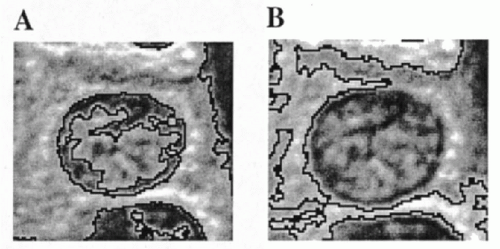 Figure 46-3 A. Segmentation by pixel OD thresholding. There is a risk of the threshold “bleeding” into the interior of the object. B. Failure of the segmentation algorithm to adhere to the object contour. |
When objects touch or overlap, one may employ a “shrink and blow” algorithm (Fig. 46-4). Here, as the pixel OD value threshold is gradually increased, an indentation appears between two overlapping objects. The indentation deepens with the increasing threshold until the objects are finally separated. The algorithm then defines a segmentation line between them and expands the two new objects to the contours of the original single object. The sequence of processing is shown in Figure 46-5A—E. Similar algorithms find cusps—sharp concavities in the outline enclosing two touching objects. The algorithm determines which two cusps best correspond to each other and positions a segmentation line accordingly. One may segment an image by enclosing or outlining areas of particular color hue.
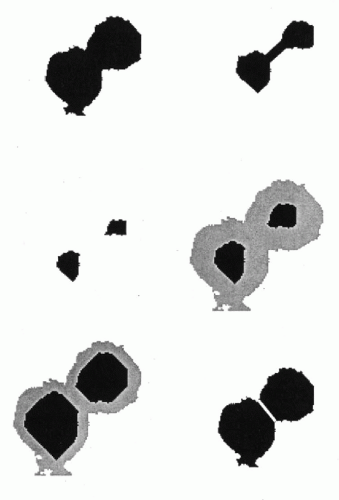 Figure 46-4 Finding of a segmentation line by a “shrink-and blow” algorithm. |
Of particular value are processing sequences based on mathematic morphologic image processing operations (Serra, 1983; Dougherty, 1992; Soille, 1998). Such operations allow all objects below a certain size to be eliminated, and the outlines of other objects to be corrected by smoothing and in-fill. The processing sequence developed by Juetting et al (1983) for the quantitative evaluation of thyroid follicles in fine needle aspirates are a good example, as shown in Figure 46-5A-E. The original image of a follicle is transformed into a histogram of pixel OD values. A threshold is set to outline nuclei. The resulting image is transformed to binary form. An erosion is performed to eliminate small particles of cellular debris and to correct small protuberances on the nuclear boundaries. By definition, a follicle includes a center or an interior region. Asearch for such interior regions is conducted within the thresholded image. The original binary image is segmented. Only the nuclei bordering the interior region are retained and stored as “follicle” for further analysis.
All these algorithms have a high success rate, but rarely does one single algorithm segment all objects correctly. An interactive correction is then required. This may be feasible when the number of objects is modest. For large images, however, full automation is mandatory, and the demanding requirements for a machine vision system have to be satisfied.
The problem of scene segmentation in cytologic preparations proved to be one of the most challenging tasks in designing automated primary screening devices for cervical cancer. It is encountered with equal degree of difficulty in karyometry in histopathologic sections. Representative regions of a lesion may extend over several square millimeters. Using objectives with high numerical aperture, this translates directly into hundreds of video frames corresponding to the number of visual fields. Interactive correction of segmentation is no longer practical.
The problem of scene segmentation in cytologic preparations proved to be one of the most challenging tasks in designing automated primary screening devices for cervical cancer. It is encountered with equal degree of difficulty in karyometry in histopathologic sections. Representative regions of a lesion may extend over several square millimeters. Using objectives with high numerical aperture, this translates directly into hundreds of video frames corresponding to the number of visual fields. Interactive correction of segmentation is no longer practical.
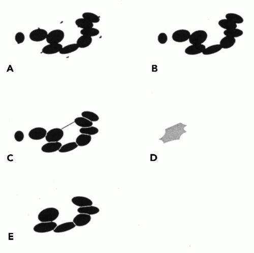 Figure 46-5 Processing of a scene by mathematical-morphologic operations. In A, the binary image of a thyroid follicle is shown. Note small debris is shown. B. The image after erosion, to remove small debris and smooth the nuclear outlines. C,D. The search for the interior region of the follicle. In E, only the nuclei forming the follicle are retained and segmentation lines are shown. |
Histometric analysis increases the degree of difficulty. One is no longer dealing with a processing task that is concerned with separate, well defined objects, such as nuclei. Instead, the histologic section is composed of adjacent components that represent a variety of structures. Processing steps to find a segmentation line for one component may adversely affect correct segmentation for other structures. The entire scene is combined or “coupled” in its processing requirements. Scene segmentation for histopathologic sections has finally become tractable by the development of knowledge-guided procedures (Liedtke et al, 1987; Thompson et al, 1993, 1995, 1996). In a knowledge-guided process, information, not offered by the image itself, is used to control the scene segmentation. This principle was first employed by Liedtke et al (1987) in the segmentation of cervical cytologic materials. Knowledge-guided process control now has been applied to the automated segmentation of prostate lesions, colonic tissues, and breast lesions (Anderson et al, 1997).
Megapixel Arrays
The first task faced in an automated analysis of histopathologic sections is the recording of the very large pixel arrays required to capture an entire diagnostically representative region (Bartels et al, 1995; Bartels et al, 1997; Ott, 1997).
For the recording of histopathologic imagery a wide field objective × 25 with a numerical aperture of 0.75 is a good choice. Such an objective typically covers a field of 750 microns in diameter, or a square image tile of around 500 microns in side length. For image sampling, the diffraction limit of the objective must be matched with the CCD elements of the video camera. Some oversampling must be allowed. This determines the choice of the relay optics (Hansen, 1986; Bartels, 1990; Baak, 1991). For a 5 × 5 mm region of a histopathologic section, this system generates 100 video frames, or an image array of 100 megapixels. Within such an array, processing and analysis of histologic structures are no longer limited by the optical image, though the seamless merging of the 100 image tiles is difficult. Two major difficulties must be controlled. First, the orientation of the CCD array and the direction of travel of the computer-controlled microscope stage must be aligned with great precision and rigidly maintained. Even so, some software adjustment during tile merging is usually required. Second, seamless joining of tiles should occur even when the merge line intersects a nucleus. These goals can be achieved by cross-correlation procedures allowing for a region of overlap (Thompson et al, 2001). Figure 46-6 shows a 100 megapixel array for a prostatic carcinoma. Images such as this are recorded at full resolution and then pixel averaged for display at different magnifications. Such images may be instantly recalled. Figure 46-7 shows a nucleus dissected by the merge line.
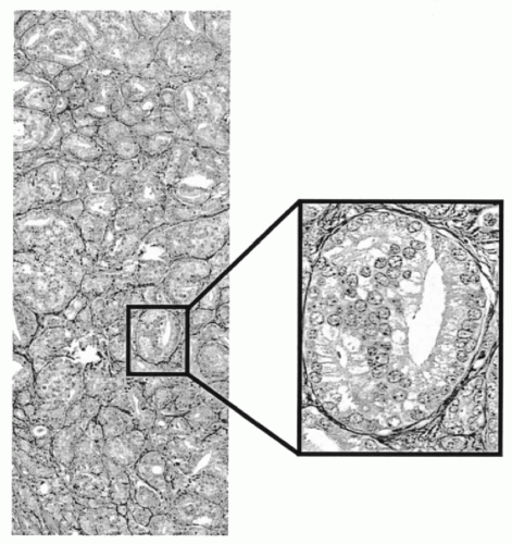 Figure 46-6 Multimegapixel array of a digitized section of prostatic carcinoma. The image is stored at full resolution, and may be recalled for any location and at any wanted reduction for display. |
Knowledge-Guided Scene Segmentation
Knowledge-guided scene segmentation provides the means for autonomous processing of imagery from a specific visual target. The knowledge-guided system should be able to segment any scene from the target in a fully automated fashion and without errors.
The principal difference between visual perception of a
microscopic image and the information evaluation by a machine vision system is that human vision perceives the entire scene simultaneously. Every object and structure is revealed in their relative position. A machine vision system acquires the data sequentially. It is “pixel-bound” in processing of the image, i.e., tied to the pixel currently being processed and its immediate neighbors. Human image assessment is supported by information not offered by the image itself, such as the professional experience of a diagnostician, knowledge of anatomy, histology, pathology, and knowledge of the relationships between structure and function. If one expects a machine vision system to perform at a comparable level, then such information must be made available to its control software. This information may be offered to the machine vision system in the form of a knowledge file (Bartels et al, 1992). A knowledge file will hold a large amount of generally applicable information, as well as very specific processing instructions for a particular and narrow diagnostic target or domain, for example, prostatic intraepithelial neoplastic lesions or a poorly differentiated prostatic carcinoma.
microscopic image and the information evaluation by a machine vision system is that human vision perceives the entire scene simultaneously. Every object and structure is revealed in their relative position. A machine vision system acquires the data sequentially. It is “pixel-bound” in processing of the image, i.e., tied to the pixel currently being processed and its immediate neighbors. Human image assessment is supported by information not offered by the image itself, such as the professional experience of a diagnostician, knowledge of anatomy, histology, pathology, and knowledge of the relationships between structure and function. If one expects a machine vision system to perform at a comparable level, then such information must be made available to its control software. This information may be offered to the machine vision system in the form of a knowledge file (Bartels et al, 1992). A knowledge file will hold a large amount of generally applicable information, as well as very specific processing instructions for a particular and narrow diagnostic target or domain, for example, prostatic intraepithelial neoplastic lesions or a poorly differentiated prostatic carcinoma.
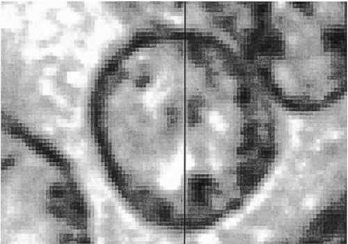 Figure 46-7 Tile merging based on cross-correlation techniques, showing the exact match of structures from both tiles down to the pixel level. |
A knowledge file consists of two major sections. In a first declarative section, all entities pertaining to a given domain are listed, with their properties, the computer operations required for their evaluation, and the sequencing of these operations. The entities entered into the knowledge file may fall into two logical groups. The first group consists of all entities recognized by the human eye, such as the nucleus, cytoplasm, various cell types, etc. The second group consists of entities that are solely related to image processing and constructs known as “intermediate segmentation products.” Examples of entities that are solely related to image processing could be red image, pixel, pixel OD value threshold and area, as well as subroutines, algorithms, and functions constructed to define a segmentation procedure, for example, a function that finds objects of interest.
Intermediate segmentation products are objects produced by machine vision segmentation during the initial processing phase aimed at detecting image regions that can be separated from the background. Some of these outlined objects may be well-defined morphologic components such as a single nucleus. Others may be objects that require further segmentation, e.g. a cluster of overlapping nuclei. Others may be fragments of one or more histologic components, such as secretory epithelium or portions of two different glands that appear in machine vision to be a single object. Figure 46-8 shows a brief processing sequence of segmentation of glandular epithelium. In Figure 46-8A, a portion of the glandular epithelium has been correctly recognized and segmented, but the gray-shaded glandular epithelium on the left belongs to three different glands. It is an intermediate segmentation product. In Figure 46-8B, the section of epithelium belonging to the gland on the lower left has been recognized, and so has the remaining segment of epithelium for the gland on the right. But, an intermediate segmentation product, now comprising segments from two different glands, still remains in need of further segmentation. Figure 46-8C indicates the segmentation line that the system found. In the next step, both of the remaining epithelial segments would be correctly assigned to their glands.
Human vision immediately identifies these intermediate segmentation products. A machine vision system needs to be given explicit instructions on how to recognize the objects and how to process them. Fortunately, only a limited number of different intermediate segmentation products occur for scenes from a given domain. They must be specified by name as separate entities in the knowledge file, to allow the control software to call on the appropriate next processing sequence.
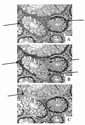 Figure 46-8 Processing sequence of a knowledge-guided segmentation. In A, the glandular epithelium from three glands remains connected, as an intermediate segmentation product. In B, the segment belonging to the gland in the right center is correctly segmented and added to that gland. In C, a portion of the epithelium belonging to the gland at the center left is correctly recognized and segmented. The glandular epithelium from the large gland at the top is assigned to that gland and a segmentation line has been drawn. |
The second section of the knowledge file contains definition statements. It gives specific processing instructions to find the required entities and also can logically relate the entities from the first two subsections to each other. The definition statements are written in a subset of English, e.g. a nucleus is an object with size (limited by constraints) and with shape (limited by constraint) and with total optical density (limited by constraint).
The knowledge file is a text file and may readily be amended or modified. It is read by the control software and consulted at run time. As the software interprets the definition statements, it sets up a node and processing sequence for each entity. The results obtained during the scene processing must satisfy the constraints at all the nodes.
Relatively simple targets or scenes, such as tissue from well-differentiated adenocarcinoma, require approximately 100 entities to allow successful segmentation for 90% to 95% of all scenes. More complex scenes have required approximately 250-300 entities to provide segmentation at the same rate of success (Thompson et al, 1995).
The complete segmentation process involves two major phases. In the first, the scene is segmented until every object is either recognized as a correctly outlined histologic entity, as listed in the knowledge file, or as a fragment of such an entity. In the second phase, the scene is reconstructed from the objects on file. In this operation, the control software has to check for logical consistency of the reconstruction. The extraction of histometric diagnostic information is begun only after scene segmentation, reconstruction and consistency checks have been completed.
A knowledge-guided scene segmentation system constitutes a major software development. The machine vision system at the Optical Sciences Center, University of Arizona, comprises some 20,000 lines of control code and image processing code. Structurally, the control software is an expert system implemented as an associated network with frames at each node (Jackson, 1986). There the specific results from the processing of each object are accumulated for later use.
Systems capable of segmenting, analyzing and interpreting imagery in a fully autonomous fashion, guided by a source of external knowledge of the domain and the processes required have become known as image understanding systems (Bartels et al, 1989).
Figure 46-9A-D shows the result of an automated segmentation of a tissue section from the prostate. Sample fields showing segmentation of lumen, stroma, secretory, and basal cell nuclei, and basal cells only are shown as a sidebar.
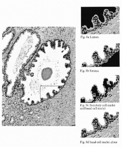 Figure 46-9 Automated segmentation of a tissue section from the prostate. The regions identified by the machine vision system as lumen, stroma, nuclei of the glandular epithelium, and basal cell nuclei alone shown in black in the small demonstration windows. Actually, the entire image is segmented automatically. |
EXTRACTION OF DIAGNOSTIC INFORMATION
With images correctly segmented and all objects of interest properly outlined, diagnostic information collection can begin with “feature extraction.”
Features
Features are descriptive entities that have numerical values. They may represent traditional diagnostic entities, such as “nuclear area” or “nucleocytoplasmic (N/C) ratio.” They may represent the spatial and statistical distribution patterns of nuclear chromatin in terms that may not have a direct visual equivalent, such as the frequency of co-occurrence of optical density (OD) values in certain range of pixels adjacent to each other. Feature extraction results in an invariant representation of an object from the image that is now characterized by a set of features.
In cytometric analysis, information of diagnostic value is offered at several different levels. There is information at the pixel level where only the properties of individual pixels are considered. This information is often used in scene segmentation to define a boundary based on pixel OD value, or pixel OD value gradient between pixels, or pixel OD value differences between images from different spectral bands.
There is information at the feature level when groups of pixels form a feature. The properties of such pixel groups are considered a feature value. The variance of all pixel OD values in a nucleus is an example.
One may transfer feature evaluation from absolute feature values to a relative scale, where all feature values are expressed in units of deviation from a “normal” reference. This makes feature evaluation less sensitive to specimen preparatory effects. Using the standard deviation of features in the normal reference data set as a unit, feature values are expressed in z-values or as relative deviation from normal.
It is customary to present all feature values in relative units because most features depend in their value on the sampling density in the image. Also, for purposes of multivariate analysis, it is advisable to have all variables of roughly the same order of magnitude.
For feature extraction from cytopathologic preparations and karyometric measurements, a set of approximately 100 features is commonly used (Bartels et al, 1980; Bengtsson et al, 1994; Doudkine et al, 1995). These features fall into distinct groups. There are features which represent an object as a whole, such as the nuclear area, total optical density, N/C ratio, variance of pixel OD values, shape features, measures of roundness of a nucleus, of concavities in the boundary or ellipticity. This group of features is often referred to as global features.
DNA PLOIDY ANALYSIS
The total optical density is one of the most often utilized global features. It is computed as the sum of all pixel optical density values within the boundary of a nucleus. It is usually expressed in arbitrary units.
Total optical density is used in dual mode, either as a descriptive feature in image analytic cell recognition, or as a quantitative cytochemical procedure, particularly DNA ploidy analysis in Feulgen-stained samples.
The Feulgen procedure (Feulgen et al, 1924) results in a stoichiometric staining of the nuclear DNA (see Chap. 44 for technical details). The total optical density measured on nuclei prepared in this fashion provides a quantitative measure of the nuclear DNA content which may be useful in diagnosis and grading of tumors (Boecking et al, 1994).
The principles of DNA ploidy measurements by image analysis are simple. The total optical density value for each individual whole nucleus is used to construct a histogram. From 100 to 1,000 nuclei, with an average of 300, must be measured to construct a reliable histogram. The distribution of the DNA values in a histogram of the unknown target is compared with the distribution of DNA values of a normal cell population. The latter may be haploid (1N) as observed in germ cells, such as human spermatozoa containing 23 chromosomes, or diploid (2N) containing double the number of chromosomes (46 in humans) as observed in all somatic cells. The number of chromosomes is proportional to DNA content. A further important variant is caused by cycling cells that double their DNA content during the S phase of the mitotic cycle. Thus, a histogram of normal DNA values of cycling diploid cells will show cells in G0G1 (2N) phase of the cell cycle, followed by gradual increase of the DNA content during the S phase, until double the original DNA content (4N) is reached during the G2M phases of the cycle, prior to cell division. Normally, the G2M peak is very small.
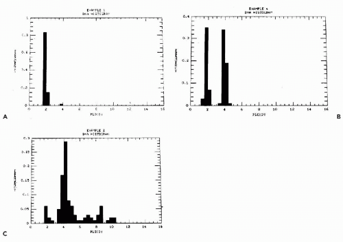 Figure 46-10 Histograms of DNA ploidy patterns in normal prostate (A), an aneuploid-tetraploid carcinoma (B), and an aneuploid carcinoma with multiple peaks (C). A shows the distribution of DNA values in normal prostate. The large peak (left) corresponds to the dominant diploid cell population in G0G1 phase of the cycle. The small peak (right) represents cells in G2M phase of the cycle. These cells are tetraploid. In B, the large peak on right shows the abnormally high number of tetraploid cells. C shows numerous peaks of abnormal DNA distribution. Histograms based on 300 cells per case. |
If the unknown sample shows a DNA distribution equal to normal, it is considered to be diploid. If the histogram of the unknown sample shows values not consistent with normal distribution, it is considered to be aneuploid. There are various forms of aneuploidy, depending on the position of the peaks. A sample can be hypo- or hyperdiploid. The latter may occur as single or multiple peaks in the histogram (Fig. 46-10). The term stemline is often used to define a single population of aneuploid cells. Thus, a tumor may have a single or multiple stemlines.
The procedure requires strict adherence to protocol (Boecking et al, 1995; Schulte, 1991). To maintain stoichiometry of staining one will have to ascertain that cells of different phenotypes, mainly reference nuclei and target nuclei, are equally affected by the hydrolysis step in the Feulgen procedure (Schulte et al, 1990). Additional problems may be experienced if attempts are made to estimate minor histogram abnormalities, such as the estimate of an S-phase fraction or detection of a near diploid stemline. In practice,
the interpretation of a DNA content histogram or “ploidy pattern” may not go farther than a visual assessment of whether aneuploidy is present.
the interpretation of a DNA content histogram or “ploidy pattern” may not go farther than a visual assessment of whether aneuploidy is present.
The most reliable results are obtained using formalin-fixed cells in smears. Measurements of DNA ploidy on tissue sections are generally not considered to be of comparable quality, or even not as acceptable at all. Corrective measures have been suggested to allow for the effects of section thickness and nuclear transection. However, even the reference nuclei used to establish the position of the 2N peak may have different sizes, geometry and orientation within the section.
Today, cell cycle analysis, S-phase fraction estimates and high-resolution stemline detection are usually performed by flow cytometry (see Chap. 47). However, image analysis is the preferred procedure when the cell sample is small, when it is essential that only tumor cells be included in the sample, by visual selection, or when one wishes to detect the presence of rare cells with abnormal DNA content.
The two methods are mutually complementary and are compared in Table 47-3 in the next chapter.
DNA ploidy measurements by image analysis have been applied to human cells and tissues, usually to elicit differences between benign and malignant tumors and differences among malignant tumors of the same origin to elicit data of prognostic value (Auer et al, 1980; Baak, 1991). In Chapter 47, the reader will find information pertaining to ploidy measurements in specific human tumors.
Pixel Optical Density Histogram
The histogram of pixel OD values typically consists of 18 features. Each of these is the relative frequency of occurrence of pixels in an optical density interval 0.10 units wide, spanning the range from OD 0 to ≥1.8. The relative frequency of occurrence of pixels in a given OD interval is a first order statistic. The count depends only on the single pixel whose value is observed. This count is not dependent on the values of other pixels in the vicinity. The pixel OD value histogram is used primarily to compare two populations. Figure 46-11 shows the histograms for a normal cell line and for a malignant cell line (Wied et al, 1968). One notes the shift of the histogram mode to high pixel OD value, in the malignant cell line, reflecting the presence of denser chromatin granules in the nuclei. The relative frequencies of occurrence of pixel OD values of nuclei are very useful in diagnostic cell classification. Their differences in a given pixel OD value interval, and the scatter about the two respective mean frequencies of occurrence, determine how well the feature “relative frequency of occurrence (dn/n) in a certain optical density interval” allows a discrimination between diagnostic categories A and B (Fig. 46-12).
Pixel OD value frequencies have been used extensively. They are robust and reliable features that reflect nuclear chromatin texture and are often the first to undergo a significant change as cells respond to changing conditions.
The pixel OD value difference histogram may be used to assess the granularity of nuclear chromatin. The pixel OD value co-occurrence matrix provides a set of features that is based on the probability that a pixel in a certain OD
value range is followed (along the scan line) by a pixel within a certain OD value range (Bartels et al, 1969; Haralick et al, 1973; Pressman, 1976). The co-occurrences are second order statistical features. Typically optical density ranges 0.30 units wide are chosen. Thus, the range from OD 0 to ≥1.8 is covered by six intervals. This yields 36 features for the co-occurrence matrix. In practice, only half of the matrix is used and the co-occurrences of pixels in ranges i,j are considered the same as from the ranges j,i. Table 46-2 shows such a co-occurrence matrix, with entries normalized to unity for the full row; here only the entries for the upper diagonal are shown.
value range is followed (along the scan line) by a pixel within a certain OD value range (Bartels et al, 1969; Haralick et al, 1973; Pressman, 1976). The co-occurrences are second order statistical features. Typically optical density ranges 0.30 units wide are chosen. Thus, the range from OD 0 to ≥1.8 is covered by six intervals. This yields 36 features for the co-occurrence matrix. In practice, only half of the matrix is used and the co-occurrences of pixels in ranges i,j are considered the same as from the ranges j,i. Table 46-2 shows such a co-occurrence matrix, with entries normalized to unity for the full row; here only the entries for the upper diagonal are shown.
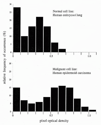 Figure 46-11 Pixel optical density histograms for a normal and a malignant cell line. Note the extension of the pixel optical density values into the higher optical density range in the malignant cells. |
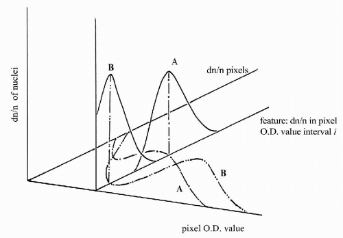 Figure 46-12 For the information offered by the pixel optical density histogram, the relative frequencies of occurrence of values in the different optical density intervals are the variables. The two horizontal axes are those relative frequencies of occurrence and the pixel optical density values. The histograms are shown for two cell types A and B. The two histograms have well separated relative frequencies of occurrence in the interval i, as shown. The vertical axis indicates the relative frequency of occurrence of nuclei having pixels in the optical density interval i, from cell type A and B. |
TABLE 46-2 CO-OCCURRENCE MATRIX | |||||
|---|---|---|---|---|---|
|


