I Sources of Variation in Medicine

Although variation in clinical medicine may be caused by biologic differences or the presence or absence of disease, it also may result from differences in the techniques and conditions of measurement, errors in measurement, and random variation. Some variation distorts data systematically in one direction, such as measuring and weighing patients while wearing shoes. This form of distortion is called systematic error and can introduce bias. Bias in turn may obscure or distort the truth being sought in a given study. Other variation is random, such as slight, inevitable inaccuracies in obtaining any measure (e.g., blood pressure). Because random error makes some readings too high and others too low, it is not systematic and does not introduce bias. However, by increasing variation in the data, random error increases the noise amidst which the signal of association, or cause and effect, must be discerned. The “louder” the noise, the more difficult it is to detect a signal and the more likely to miss an actual signal. All these issues are revisited here and in subsequent chapters. The sources of variation are illustrated in this chapter using the measurement of blood pressure in particular.

Biologic differences include factors such as differences in genes, nutrition, environmental exposures, age, gender, and race. Blood pressure tends to be higher among individuals with high salt intake, in older persons, and in persons of African descent. Tall parents usually have tall children. Extremely short people may have specific genetic conditions (e.g., achondroplasia) or a deficiency of growth hormone. Although poor nutrition slows growth, and starvation may stop growth altogether, good nutrition allows the full genetic growth potential to be achieved. Polluted water may cause intestinal infections in children, which can retard growth, partly because such infections exacerbate malnutrition.

Variation is seen not only in the presence or absence of disease, but also in the stages or extent of disease. Cancer of the cervix may be in situ, localized, invasive, or metastatic. In some patients, multiple diseases may be present (comorbidity). For example, insulin-dependent diabetes mellitus may be accompanied by coronary artery disease or renal disease.

Different conditions of measurement often account for the variations observed in medical data and include factors such as time of day, ambient temperature or noise, and the presence of fatigue or anxiety in the patient. Blood pressure is higher with anxiety or following exercise and lower after sleep. These differences in blood pressure are not errors of measurement, but of standardizing the conditions under which the data are obtained. Standardizing such conditions is important to avoid variation attributable to them and the introduction of bias.

Different techniques of measurement can produce different results. A blood pressure (BP) measurement derived from the use of an intra-arterial catheter may differ from a measurement derived from the use of an arm cuff. This may result from differences in the measurement site (e.g., central or distal arterial site), thickness of the arm (which influences reading from BP cuff), rigidity of the artery (reflecting degree of atherosclerosis), and interobserver differences in the interpretation of BP sounds.

Some variation is caused by measurement error. Two different BP cuffs of the same size may give different measurements in the same patient because of defective performance by one of the cuffs. Different laboratory instruments or methods may produce different readings from the same sample. Different x-ray machines may produce films of varying quality. When two clinicians examine the same patient or the same specimen (e.g., x-ray film), they may report different results¹ (see Chapter 7). One radiologist may read a mammogram as abnormal and recommend further tests, such as a biopsy, whereas another radiologist may read the same mammogram as normal and not recommend further workup.² One clinician may detect a problem such as a retinal hemorrhage or a heart murmur, and another may fail to detect it. Two clinicians may detect a heart murmur in the same patient but disagree on its characteristics. If two clinicians are asked to characterize a dark skin lesion, one may call it a “nevus,” whereas the other may say it is “suspicious for malignant melanoma.” A pathologic specimen would be used to resolve the difference, but that, too, is subject to interpretation, and two pathologists might differ.

Variation seems to be a ubiquitous phenomenon in clinical medicine and research. Statistics can help investigators to interpret data despite biologic variation, but statistics cannot correct for errors in the observation or recording of data. Stated differently, statistics can compensate for random error in a variety of ways, but statistics cannot fix, “after the fact” (post hoc), bias introduced by systematic error.

II Statistics and Variables

Statistical methods help clinicians and investigators understand and explain the variation in medical data. The first step in understanding variation is to describe it. This chapter focuses on how to describe variation in medical observations. Statistics can be viewed as a set of tools for working with data, just as brushes are tools used by an artist for painting. One reason for the choice of a specific tool over another is the type of material with which the tool would be used. One type of brush is needed for oil paints, another for tempera paints, and another type for watercolors. The artist must know the materials to be used to choose the correct tools. Similarly, a person who works with data must understand the different types of variables that exist in medicine.

B Types of Variables

Variables can be classified as nominal variables, dichotomous (binary) variables, ordinal (ranked) variables, continuous (dimensional) variables, ratio variables, and risks and proportions (Table 9-1).

Table 9-1 Examples of the Different Types of Data

Information Content	Variable Type	Examples
Higher	Ratio	Temperature (Kelvin); blood pressure*
	Continuous (dimensional)	Temperature (Fahrenheit)*
	Ordinal (ranked)	Edema = 3+ out of 5 Perceived quality of care = good/fair/poor
	Binary (dichotomous)	Gender; heart murmur = present/absent
	Nominal	Blood type; color = cyanotic or jaundiced; taste = bitter or sweet
Lower

Note: Variables with higher information content may be collapsed into variables with less information content. For example, hypertension could be described as “165/95 mm Hg” (continuous data), “absent/mild/moderate/severe” (ordinal data), or “present/absent” (binary data). One cannot move in the other direction, however. Also, knowing the type of variables being analyzed is crucial for deciding which statistical test to use (see Table 11-1).

^*For most types of data analysis, the distinction between continuous data and ratio data is unimportant. Risks and proportions sometimes are analyzed using the statistical methods for continuous variables, and sometimes observed counts are analyzed in tables, using nonparametric methods (see Chapter 11).

1 Nominal Variables

Nominal variables are “naming” or categorical variables that have no measurement scales and no rank order. Examples are blood groups (O, A, B, and AB), occupations, food groups, and skin color. If skin color is the variable being examined, a different number can be assigned to each color (e.g., 1 is bluish purple, 2 is black, 3 is white, 4 is blue, 5 is tan) before the information is entered into a computer data system. Any number could be assigned to any color, and that would make no difference to the statistical analysis. This is because the number is merely a numerical name for a color, and size of the number used has no inherent meaning; the number given to a particular color has nothing to do with the quality, value, or importance of the color.

2 Dichotomous (Binary) Variables

If all skin colors were included in one nominal variable, there is a problem: the variable does not distinguish between normal and abnormal skin color, which is usually the most important aspect of skin color for clinical and research purposes. As discussed, abnormal skin color (e.g., pallor, jaundice, cyanosis) may be a sign of numerous health problems (e.g., anemia, liver disease, cardiac failure). Researchers might choose to create a variable with only two levels: normal skin color (coded as a 1) and abnormal skin color (coded as a 2). This new variable, which has only two levels, is said to be dichotomous (Greek, “cut into two”).

Many dichotomous variables, such as well/sick, living/dead, and normal/abnormal, have an implied direction that is favorable. Knowing that direction would be important for interpreting the data, but not for the statistical analysis. Other dichotomous variables, such as female/male and treatment/placebo, have no a priori qualitative direction.

Dichotomous variables, although common and important, often are inadequate by themselves to describe something fully. When analyzing cancer therapy, it is important to know not only whether the patient survives or dies (a dichotomous variable), but also how long the patient survives (time forms a continuous variable). A survival analysis or life table analysis, as described in Chapter 11, may be done. It is important to know the quality of patients’ lives while they are receiving the therapy; this might be measured with an ordinal variable, discussed next. Similarly, for a study of heart murmurs, various types of data may be needed, such as dichotomous data concerning a murmur’s timing (e.g., systolic or diastolic), nominal data on its location (e.g., aortic valve area) and character (e.g., rough), and ordinal data on its loudness (e.g., grade III). Dichotomous variables and nominal variables sometimes are called discrete variables because the different categories are completely separate from each other.

3 Ordinal (Ranked) Variables

Many types of medical data can be characterized in terms of three or more qualitative values that have a clearly implied direction from better to worse. An example might be “satisfaction with care” that could take on the values of “very satisfied,” “fairly satisfied,” or “not satisfied.” These data are not measured on a measurement scale. They form an ordinal (i.e., ordered or ranked) variable.

There are many clinical examples of ordinal variables. The amount of swelling in a patient’s legs is estimated by the clinician and is usually reported as “none” or 1+, 2+, 3+, or 4+ pitting edema (puffiness). A patient may have a systolic murmur ranging from 1+ to 6+. Respiratory distress is reported as being absent, mild, moderate, or severe. Although pain also may be reported as being absent, mild, moderate, or severe, in most cases, patients are asked to describe their pain on a scale from 0 to 10, with 0 being no pain and 10 the worst imaginable pain. The utility of such scales to quantify subjective assessments such as pain intensity is controversial and is the subject of ongoing research.

Ordinal variables are not measured on an exact measurement scale, but more information is contained in them than in nominal variables. It is possible to see the relationship between two ordinal categories and know whether one category is more desirable than another. Because they contain more information than nominal variables, ordinal variables enable more informative conclusions to be drawn. As described in Chapter 11, ordinal variables often require special techniques of analysis.

4 Continuous (Dimensional) Variables

Many types of medically important data are measured on continuous (dimensional) measurement scales. Patients’ heights, weights, systolic and diastolic blood pressures, and serum glucose levels all are examples of data measured on continuous scales. Even more information is contained in continuous data than in ordinal data because continuous data not only show the position of the different observations relative to each other, but also show the extent to which one observation differs from another. Continuous data often enable investigators to make more detailed inferences than do ordinal or nominal data.

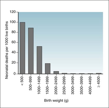
Relationships between continuous variables are not always linear (in a straight line). The relationship between the birth weight and the probability of survival of newborns is not linear.³ As shown in Figure 9-1, infants weighing less than 3000 g and infants weighing more than 4500 g are historically at greater risk for neonatal death than are infants weighing 3000 to 4500 g (~6.6-9.9 lb).

Figure 9-1 Histogram showing neonatal mortality rate by birth weight group, all races, United States, 1980.

(Data from Buehler JW et al: Public Health Rep 102:151–161, 1987.)

5 Ratio Variables

If a continuous scale has a true 0 point, the variables derived from it can be called ratio variables. The Kelvin temperature scale is a ratio scale because 0 degrees on this scale is absolute 0. The centigrade temperature scale is a continuous scale, but not a ratio scale because 0 degrees on this scale does not mean the absence of heat. For some purposes, it may be useful to know that 200 units of something is twice as large as 100 units, information provided only by a ratio scale. For most statistical analyses, however, including significance testing, the distinction between continuous and ratio variables is not important.

6 Risks and Proportions as Variables

As discussed in Chapter 2, a risk is the conditional probability of an event (e.g., death or disease) in a defined population in a defined period. Risks and proportions, which are two important types of measurement in medicine, share some characteristics of a discrete variable and some characteristics of a continuous variable. It makes no conceptual sense to say that a “fraction” of a death occurred or that a “fraction” of a person experienced an event. It does make sense, however, to say that a discrete event (e.g., death) or a discrete characteristic (e.g., presence of a murmur) occurred in a fraction of a population. Risks and proportions are variables created by the ratio of counts in the numerator to counts in the denominator. Risks and proportions sometimes are analyzed using the statistical methods for continuous variables (see Chapter 10), and sometimes observed counts are analyzed in tables, using statistical methods for analyzing discrete data (see Chapter 11).

C Counts and Units of Observation

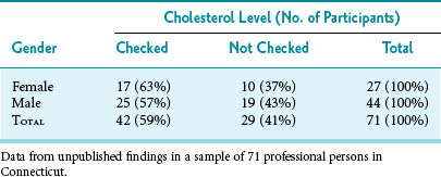
The unit of observation is the person or thing from which the data originated. Common examples of units of observation in medical research are persons, animals, and cells. Units of observation may be arranged in a frequency table, with one characteristic on the x-axis, another characteristic on the y-axis, and the appropriate counts in the cells of the table. Table 9-2, which provides an example of this type of 2 × 2 table, shows that among 71 young professional persons studied, 63% of women and 57% of men previously had their cholesterol levels checked. Using these data and the chi-square test described in Chapter 11, one can determine whether or not the difference in the percentage of women and men with cholesterol checks was likely a result of chance variation (in this case the answer is “yes”).

Table 9-2 Standard 2 × 2 Table Showing Gender of 71 Participants and Whether or Not Serum Total Cholesterol Was Checked

III Frequency Distributions

A Frequency Distributions of Continuous Variables

Observations on one variable may be shown visually by putting the variable’s values on one axis (usually the horizontal axis or x-axis) and putting the frequency with which that value appears on the other axis (usually the vertical axis or y-axis). This is known as a frequency distribution. Table 9-3 and Figure 9-2 show the distribution of the levels of total cholesterol among 71 professional persons. The figure is shown in addition to the table because the data are easier to interpret from the figure.

Table 9-3 Serum Levels of Total Cholesterol Reported in 71 Participants^*

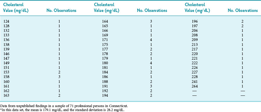
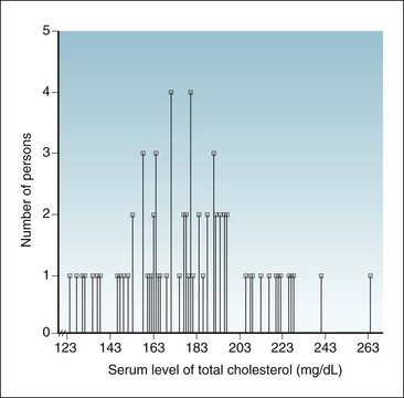
Figure 9-2 Histogram showing frequency distribution of serum levels of total cholesterol.
As reported in a sample of 71 participants; data shown here are same data listed in Table 9-3; see also Figures 9-4 and 9-5.

(Data from unpublished findings in a sample of 71 professional persons in Connecticut.)

Only gold members can continue reading. Log In or Register to continue

You may also need

• The Study of Risk Factors and Causation
• Bivariate Analysis
• Birth Outcomes: A Global Perspective
• Clinical Preventive Services (United States Preventive Services Task Force)
• Assessment of Risk and Benefit in Epidemiologic Studies
• Common Research Designs and Issues in Epidemiology
• Epidemiologic Data Measurements
• Disaster Epidemiology and Surveillance

Share this:

• Click to share on Twitter (Opens in new window)
• Click to share on Facebook (Opens in new window)
• Click to share on Google+ (Opens in new window)

Like this:

Like Loading...

Related