6 Assessment of Risk and Benefit in Epidemiologic Studies

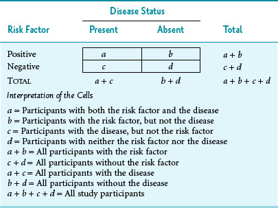
Despite these complexities, much epidemiologic research still relies on the dichotomies of exposed/unexposed and diseased/nondiseased, which are often presented in the form of a standard 2 × 2 table (Table 6-1).
II Comparison of Risks in Different Study Groups
Although differences in risk can be measured in absolute terms or in relative terms, the method used depends on the type of study performed. For reasons discussed in Chapter 5, case-control studies allow investigators to obtain only a relative measure of risk, whereas cohort studies and randomized controlled trials allow investigators to obtain absolute and relative measures of risk. Whenever possible, it is important to examine absolute and relative risks because they provide different information.
After the differences in risk are calculated by the methods outlined in detail subsequently, the level of statistical significance must be determined to ensure that any observed difference is probably real (i.e., not caused by chance). (Significance testing is discussed in detail in Chapter 10.) When the difference is statistically significant, but not clinically important, it is real but trivial. When the difference appears to be clinically important, but is not statistically significant, it may be a false-negative (beta) error if the sample size is small (see Chapter 12), or it may be a chance finding.
A Absolute Differences in Risk
Disease frequency usually is measured as a risk in cohort studies and clinical trials and as a rate when the disease and death data come from population-based reporting systems. An absolute difference in risks or rates can be expressed as a risk difference or as a rate difference. The risk difference is the risk in the exposed group minus the risk in the unexposed group. The rate difference is the rate in the exposed group minus the rate in the unexposed group (rates are defined in Chapter 2). The discussion in this chapter focuses on risks, which are used more often than rates in cohort studies.
In Table 6-1 the risk of disease in the exposed individuals is a/(a + b), and the risk of disease in the unexposed individuals is c/(c + d). When these symbols are used, the attributable risk (AR) can be expressed as the difference between the two:
Figure 6-1 provides data on age-adjusted death rates for lung cancer among adult male smokers and nonsmokers in the U.S. population in 1986 and in the United Kingdom (UK) population.1,2 For the United States in 1986, the lung cancer death rate in smokers was 191 per 100,000 population per year, whereas the rate in nonsmokers was 8.7 per 100,000 per year. Because the death rates for lung cancer in the population were low (<1% per year) in the year for which data are shown, the rate and the risk for lung cancer death would be essentially the same. The risk difference (attributable risk) in the United States can be calculated as follows:
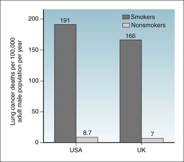
Figure 6-1 Risk of death from lung cancer.
Comparison of the risks of death from lung cancer per 100,000 adult male population per year for smokers and nonsmokers in the United States (USA) and United Kingdom (UK).
(Data from US Centers for Disease Control: MMWR 38:501–505, 1989; and Doll R, Hill AB: BMJ 2:1071–1081, 1956.)

Similarly, the attributable risk in the UK can be calculated as follows:

B Relative Differences in Risk
1 Relative Risk (Risk Ratio)
The relative risk, which is also known as the risk ratio (both abbreviated as RR), is the ratio of the risk in the exposed group to the risk in the unexposed group. If the risks in the exposed group and unexposed group are the same, RR = 1. If the risks in the two groups are not the same, calculating RR provides a straightforward way of showing in relative terms how much different (greater or smaller) the risks in the exposed group are compared with the risks in the unexposed group. The risk for the disease in the exposed group usually is greater if an exposure is harmful (as with cigarette smoking) or smaller if an exposure is protective (as with a vaccine). In terms of the groups and symbols defined in Table 6-1, relative risk (RR) would be calculated as follows:
The data on lung cancer deaths in Figure 6-1 are used to determine the attributable risk (AR). The same data can be used to calculate the RR. For men in the United States, 191/100,000 divided by 8.7/100,000 yields an RR of 22. Figure 6-2 shows the conversion from absolute to relative risks. Absolute risk is shown on the left axis and relative risk on the right axis. In relative risk terms the value of the risk for lung cancer death in the unexposed group is 1. Compared with that, the risk for lung cancer death in the exposed group is 22 times as great, and the attributable risk is the difference, which is 182.3/100,000 in absolute risk terms and 21 in relative risk terms.
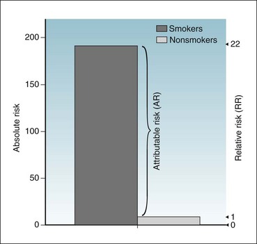
Figure 6-2 Risk of death from lung cancer.
Diagram shows the risks of death from lung cancer per 100,000 adult male population per year for smokers and nonsmokers in the United States, expressed in absolute terms (left axis) and in relative terms (right axis).
(Data from US Centers for Disease Control: MMWR 38:501–505, 1989.)
2 Odds Ratio
People may be unfamiliar with the concept of odds and the difference between “risk” and “odds.” Based on the symbols used in Table 6-1, the risk of disease in the exposed group is a/(a + b), whereas the odds of disease in the exposed group is simply a/b. If a is small compared with b, the odds would be similar to the risk. If a particular disease occurs in 1 person among a group of 100 persons in a given year, the risk of that disease is 1 in 100 (0.0100), and the odds of that disease are 1 to 99 (0.0101). If the risk of the disease is relatively large (>5%), the odds ratio is not a good estimate of the risk ratio. The odds ratio can be calculated by dividing the odds of exposure in the diseased group by the odds of exposure in the nondiseased group. In the terms used in Table 6-1, the formula for the OR is as follows:
In mathematical terms, it would make no difference whether the odds ratio was calculated as (a/c)/(b/d) or as (a/b)/(c/d) because cross-multiplication in either case would yield ad/bc. In a case-control study, it makes no sense to use (a/b)/(c/d) because cells a and b come from different study groups. The fact that the odds ratio is the same whether it is developed from a horizontal analysis of the table or from a vertical analysis proves to be valuable, however, for analyzing data from case-control studies. Although a risk or a risk ratio cannot be calculated from a case-control study, an odds ratio can be calculated. Under most real-world circumstances, the odds ratio from a carefully performed case-control study is a good estimate of the risk ratio that would have been obtained from a more costly and time-consuming prospective cohort study. The odds ratio may be used as an estimate of the risk ratio if the risk of disease in the population is low. (It can be used if the risk ratio is <1%, and probably if <5%.) The odds ratio also is used in logistic methods of statistical analysis (logistic regression, log-linear models, Cox regression analyses), discussed briefly in Chapter 13.
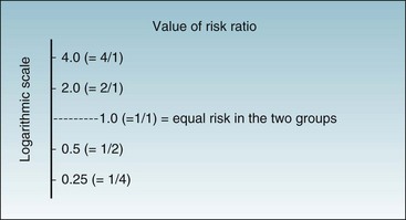
3 Which Side Is Up in the Risk Ratio and Odds Ratio?
Another risk factor might produce 4 times the risk of a disease, in which case the ratio could be expressed as 4 or as 1/4, depending on how the risks are being compared. When the risk ratio is plotted on a logarithmic scale (Fig. 6-3), it is easy to see that, regardless of which way the ratio is expressed, the distance to the risk ratio of 1 is the same. Mathematically, it does not matter whether the risk for the exposed group or the unexposed group is in the numerator. Either way the risk ratio is easily interpretable. Almost always the risk of the exposed group is expressed in the numerator, however, so that the numbers make intuitive sense.
Stay updated, free articles. Join our Telegram channel

Full access? Get Clinical Tree


