and Jordan Smoller2
(1)
Department of Epidemiology, Albert Einstein College of Medicine, Bronx, NY, USA
(2)
Department of Psychiatry and Center for Human Genetic Research, Massachusetts General Hospital, Boston, MA, USA
Let us then suppose the mind to be, as we say, white paper (tabula rasa), void of all characters without any ideas; how comes it to be furnished? Whence comes it by that vast store, which the busy and boundless fancy of man has painted on it with an almost endless variety?….To this I answer, in one word, From experience: in that all our knowledge is founded….
John Locke
An Essay Concerning Human Understanding (1689)
8.1 A New Scientific Era
We are a long way from believing that the mind is a “tabula rasa,” a blank slate. We know now that much is in fact innate, i.e., under genetic influence. The purpose of this chapter is to help those who wish to read the rapidly expanding literature in genetic epidemiology. Thus, it is an overview of the basic designs and statistics used in this area; it is not comprehensive, nor is it highly technical.
The focus of epidemiological research has evolved as parallel progress has been made in other fields of medicine and basic science. In the era when infectious diseases were rampant, epidemiology was concerned with identifying the sources of the infection and methods of transmission, largely through fieldwork. As the infectious agents were discovered, as sanitation and health status improved, chronic diseases, such as heart disease and cancer, became the leading causes of death and disability in the developed world and came to be the foremost targets of epidemiological research. (Now that new infectious diseases are once again emerging, this part of epidemiology is again gaining prominence).
The objective of chronic disease epidemiology was to identify risk factors for these diseases. This part of the story has been a great public health success. We now know, because of epidemiological studies, what the major modifiable risk factors are for cardiovascular disease: hypertension, high cholesterol and LDL, smoking, overweight, and inactivity. Our challenge now is to find ways to make the lifestyle changes in the population, which will further lower the rates of cardiovascular disease. We also know many of the exposures related to cancer, but not as comprehensively as for heart disease.
At this scientifically historic time, as science is fully entering into the era of genomics, epigenomics, and proteomics (and other “omics”), epidemiology has entered a new phase of research activity: molecular epidemiology. This is the search for blood or tissue biomarkers and genetic polymorphisms (variants) that are associated with or predispose to disease. Why is this different from any other risk factor investigated in epidemiology? In many ways it isn’t, especially with regard to the blood biomarkers, but in genetic epidemiology, there are study designs and statistical analysis methods that are quite different. A really new aspect of molecular and genetic epidemiology is the true collaboration of basic scientists, clinicians, and epidemiologists. For too long the disciplines have gone their separate research ways and scientists read mostly the scientific journals in their own field. But molecular epidemiology cannot fruitfully proceed without the interface of laboratory scientists and population researchers.
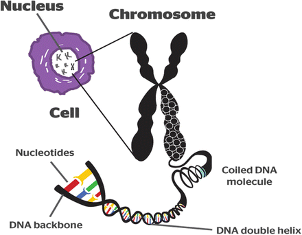
Below are some basics of genetics which you can skip reading if this is all familiar. DNA (deoxyribonucleic acid) is made up of four units—or nucleotides. These nucleotides, also called bases, are adenine, guanine, thymine, and cytosine and are denoted by the letters A, G, T, and C. The DNA is arranged in two strands twisted in a double helix form, such that the nucleotides AGCT pair with each other in fixed ways. An A always pairs with T and C always pairs with G. These are called base pairs. If one strand of the double helix were strung out in a line, it might look like this:
AATTCGTCAGTCCC. The other strand that pairs with it would be
TTAAGCAGTCAGGG.
There are three billion base pairs (or six billion bases) in the human genome (which refers to all the genetic material in humans). These three billion base pairs are organized into 23 chromosome pairs (one from the mother and one from the father), which are in every living cell in the body (except the sperm and egg cells each of which have 1 chromosome each until they merge to form a fertilized cell that now has the full complement of chromosomes). Within these three billion base pairs, there are about 20,000 genes which are sequences of base pairs of different lengths and which provide the code for the formation of proteins. The remaining sequences serve mostly regulatory functions or have functions that are unknown at the present time. The most common variations in the genome are known as single nucleotide polymorphisms (SNPs, pronounced as “snips”) and involve a difference in a single letter of the genetic code. Some SNPs are normal variants in a population, some may protect against disease, and some may predispose to disease.
8.2 Overview of Genetic Epidemiology
Genetic epidemiology seeks to identify genes related to disease and to assess the impact of genetic factors on population health and disease. Here is an overview of the strategy often used to study genetic determinants of disease. First we may want to determine if the disease runs in families. If it is not familial, it is not likely to be heritable; if it is familial, it may or may not be due to genetic factors (environments run in families also). Next, we want to see if genetic variation contributes to the familial transmission. One method for determining this is by studying twins (described in Section 8.3). If we determine the disease is heritable, we would want to localize and identify the genes involved. And finally, we want to understand the mechanisms by which these genes contribute to disease.
As a first step, we may want to find out where the genes that contribute to the disorder are located. One approach to this is to conduct linkage studies of individuals affected with the disease and their families (described in Section 8.4). Linkage studies may identify regions on the chromosome that are likely to harbor the disease genes. Once we’ve identified one or more such regions, we may look to see what genes are known to reside in those regions. We can then test these genes using association studies in unrelated individuals (described in Section 8.6) to determine whether any variants (also called alleles) of these genes are associated with the disease. Another approach, better suited to common complex diseases, is to begin with genomewide association studies (discussed in Section 8.10).
So, there are a variety of designs and statistical tests that can be used to define the genetic basis of a disease, including (1) twin studies to determine if the disease has a heritable component; (2) linkage studies to identify and locate regions of chromosomes containing genes involved in the disease; and (3) association studies to determine whether specific genetic variants are associated with the disease, to examine how they interact with the environment, and to determine how they affect population health. We will limit the discussion to some pretty simple models that will give the flavor of the topic. Readers interested in more depth are referred to the many more technical writings on the subject, listed in the reference 31 – 35section for this chapter.
8.3 Twin Studies
To explore a genetic influence on disease, we may first look to see if it runs in families. But something that is familial is not necessarily heritable. For example: do obese parents have obese children because of genetics or because of nutrition and activity levels that are transmitted from the parents to the children? What we want to know is whether and to what extent the phenotype (what we observe in the person, e.g., obesity) is affected by genetic factors.
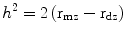
One way to assess the influence of genetic variation is from studies of twins. Identical twins (monozygotic—coming from the same fertilized egg) share 100 % of their genes, while fraternal twins (dizygotic—coming from two fertilized eggs) share on average 50 %, just as non-twin siblings do. One way to estimate the strength of genetic influences is to calculate the heritability, h 2. For twin studies, heritability can be calculated as twice the difference between the correlation for that trait among monozygotic twins minus the correlation in dizygotic twins or
 Consider blood pressure. If variation in the condition or trait under investigation were completely attributable to genetic variation, then each member of a monozygotic twin pair would be equally affected (each member would have the same blood pressure) and the correlation between monozygotic twins would be 1.0; the correlation in dizygotic twins, however, would be .50.
In this case, h 2 would be 2(1–0.5) = 1.0 or 100 %. If the condition is completely not heritable in the population, then rmz = rdz and h 2 = 0. Since diseases and traits are generally partially heritable, h 2 lies somewhere between 0 and 1.0.
If we are talking about continuous variables, we can think of heritability in terms of correlation coefficients. If we are talking about categorical variables, we may speak of concordance rates, where
 Some reported approximate estimates31 – 33 of heritability from twin studies are .60 for alcoholism, .30–.50 for personality traits, .35 for colorectal cancer, .26 for multiple sclerosis, 0.75 for height, and .80 for schizophrenia.
It is important to remember that heritability doesn’t measure how much of an individual’s disease is attributable to genetics; rather it tells us what proportion of the population’s variability in the phenotype is the result of variation in the genes in the population. So it is a measure applicable to a population, not to an individual. If you have people living in exactly the same environment, then any variation you encounter in the phenotype would be mainly due to genetic factors, since there is no environmental variation. In such a case, if all environmental factors are constant for the population, heritability would be 100 %. So there are some limitations to this measure, but it does give us an idea to what extent genetic variation contributes to phenotypic variation in a population. However, heritability tells us nothing about what genes are responsible for that variation, which genetic variants are involved, how many variants are involved, or what their effect sizes are. This more detailed information is referred to as the “genetic architecture” of a trait or disease.
8.4 Linkage and Association Studies
If we know that a disease is heritable, we can now turn to the task of actually identifying the genes that are involved. Most disorders that are studied by epidemiologists (e.g., cardiovascular diseases, psychiatric disorders, common forms of cancer) are considered “complex” disorders. Unlike single-gene or Mendelian disorders, such as cystic fibrosis or Huntington’s disease, complex disorder diseases are thought to result from the contribution of several or many genes interacting with environmental risk factors. That can make identifying the effect of an individual gene quite a difficult task. The effect of a particular allele within that gene may be quite small. It is a bit like looking for the proverbial needle in the haystack. Nevertheless, genes contributing to diseases are being discovered and there are certain strategies that are employed in the search.
Where in the genome do we look for the genes that confer susceptibility to the disease? One way to answer this question is to use genetic linkage analysis.
(a)
Linkage analysis relies on the phenomena of crossing over and recombination that occur during the process of meiosis when the sex cells (sperm and egg) are formed. Each person has two copies of each of the 23 chromosomes that make up the genome: one copy is inherited from the mother and one from the father. During the formation of sperm and egg cells, these 23 chromosome pairs line up and exchange segments of genetic material in a process known as crossing over. This recombination occurs at one or more places along the chromosome. The closer two loci are on a chromosome, the less likely a recombination event will occur between them and so the more likely they will be inherited together. Loci that tend to be co-inherited are said to be genetically linked. We can use this fact to estimate the distance between two genetic loci or markers (a genetic marker is a DNA variation whose chromosomal location is known). The physical distance between two markers is inversely related to how frequently they are co-inherited across generations in a family.
(b)
The distance between two loci is sometimes measured in centimorgans. A centimorgan (cM) is a unit of distance along a chromosome, but not in the ordinary sense of physical distance. It is really a probability measure which is a reflection of the physical distance; it reflects the probability of two markers or loci being separated (or segregated) by crossing over during meiosis. If the two markers are very close together, they won’t separate (we say they are “linked”); if they are far apart, they are likelier to cross over and the genetic material gets recombined during meiosis. Then this recombined DNA gets transmitted to the offspring. Two loci are one centimorgan apart if the probability that they are separated by crossing over is only 1 % (once in a hundred meioses). It has been estimated that there are about 1 million base pairs in a 1 cM span. Loci that are far apart, say 50 cM, will be inherited independently of each other, as they would be if they were on different chromosomes. The purpose of linkage studies is to localize the disease susceptibility gene to be within some region on the chromosome.
(c)
So we might begin our search for a disease gene by collecting families affected by the disease and performing a linkage analysis using markers spaced at intervals (say 10 cM apart) across the entire genome. If we find a marker that appears to be co-transmitted with the disease, we would have evidence that the marker is genetically linked to a gene for the disease. In other words, there is likely to be a gene for the disease in the same region as the linked marker.
(d)
Having found a chromosomal region linked to the disease, we might try to narrow the region down by genotyping and testing additional markers within that region (say at 1 cM intervals). However, even this relatively small region may contain many genes.
(e)
Our next step might be to screen the genes that are known to reside in this region. We would be particularly interested in genes that have a plausible connection to the disease of interest (these would be good “candidate genes”). For example, if we are studying diabetes, genes that make proteins involved in glucose metabolism would be important “candidate genes.”
(f)
Now we can see if any particular alleles (variants) of the genes in that chromosomal region are associated with the disease. This can be done by:
(1)
Association studies using case–control methods in unrelated people, examining whether an allele is more common in cases than controls (described in Sect. 8.6)
(2)
Association studies in families to see whether an allele is being transmitted more commonly to cases than expected by chance (described in Sect. 8.9)
So, essentially, linkage analysis tells us that a particular marker location is near a disease susceptibility gene; association analysis tells us that a particular allele of a gene or marker is more commonly inherited by individuals with the disease.
8.5 LOD Score: Linkage Statistic
The classic statistic used to evaluate the strength of the evidence in favor of linkage of a genetic marker and disease susceptibility gene is the LOD score (the log10 of the odds in favor of linkage). It will be described in principle only, to help in interpretation of epidemiological articles dealing with genetics. The actual calculations are complex and require special program packages.
The principle underlying the LOD score is described in the previous section: if we have two loci—say, a marker and a disease gene—the closer they are on a chromosome, the lower the probability that they will be separated by a recombination event during meiosis and the more likely they will be co-inherited by offspring.
The probability of recombination, called the recombination fraction, is denoted by the symbol θ and depends on the distance between the gene and the marker. If there is no recombination and the gene and marker are completely linked, then the recombination fraction is 0. The maximum value of θ is .5 (if gene and marker were independently inherited, then the probability that the marker was transmitted but not the gene = the probability that gene was transmitted but not the marker = .50).
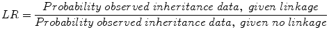
So if you want to know if there is linkage, we have to estimate how likely it is that θ is less than .5, given the data we have observed. We use the likelihood ratio for this, which as you recall from Chapter 2 is the ratio of the probability of observed symptoms, given disease divided by the probability of observed symptoms given no disease. In this case
 The null hypothesis here is no linkage (or recombination fraction θ = .5) and the alternate hypothesis is linkage (or θ < .5). If we reject the null, we “accept” the alternate hypothesis. The test statistics used to see if we have sufficient data to conclude linkage is the LOD score which is the log 10 (LR). For Mendelian (single-gene) disorders, a LOD score of 3 has traditionally been the threshold for declaring significant linkage, although for complex disorders higher thresholds (3.3–3.6) have been recommended. A LOD score of 3.0 indicates 103 odds in favor of linkage compared to no linkage, i.e., 1,000:1 odds in favor of linkage.
For complex reasons beyond the scope of this book (but described in the references at the end), a LOD score can be translated into probability by multiplying it by the constant 4.6: LOD × 4.6 is distributed as chi-square with 1 degree of freedom. (The 4.6 is 2 times the natural log of 10.) Thus, a LOD of 3.0 is equivalent to a chi-square of 3 × 4.6 = 13.82 and corresponds to p = .0002. The inheritance data for linkage analyses can come from family pedigree studies, from sibships or other family groups.
LOD score linkage analysis is sometimes referred to as “parametric” linkage analysis because it requires that we specify certain parameters (e.g., disease and marker allele frequencies, recessive vs. dominant mode of inheritance, penetrance of the disease gene). When these parameters are known or can be approximated, parametric LOD score analysis is the most powerful method of linkage analysis. This may be true for Mendelian (single-gene) disease, but for many complex disorders, these parameters are not known. “Nonparametric” linkage methods (known as the allele-sharing approach) are often used to study complex disorders because they do not require knowledge of the mode of inheritance or other genetic parameters. There are a number of statistics available, described in the more advanced texts.
8.6 Association Studies
Compared to linkage analysis, association studies are more closely akin to traditional epidemiological studies and most often rely on the case–control design. In an association study, investigators are interested in finding whether there is any association between a particular allele at a polymorphic locus and the phenotype in question. (A polymorphism is a variation in DNA sequence that occurs in at least 1 % of the population. A variation that occurs in less than 1 % is referred to as a mutation). For the purposes of this discussion, we will assume that the polymorphisms we are looking at are SNPs (single nucleotide polymorphisms) or variants in a single one of the bases A, T, C, G (standing for adenine, thymine, guanine, cytosine) at a particular locus. Note that there are many other classes of DNA variation including small insertions and deletions of nucleotides and copy number variations that involve deletion or duplication of larger chunks of DNA, as illustrated below.
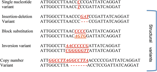
Reprinted by permission from Macmillan Publishers Ltd: [Nature Reviews Genetics] (Frazer KA, Murray SS, Schork NJ, Topol EJ, Human genetic variation and its contribution to complex traits), copyright (2009)
So let us say at a particular SNP some people have the A allele and other people have the G allele. We want to know if people with the disease are more likely to have say, the A allele than the G allele. For a binary phenotype (e.g., diseased or not), we can do case–control studies of association by taking cases who are affected with the disease and unrelated controls who are not. Remember that each person gets one copy of an allele at a particular locus from the mother and one copy from the father. (These are exactly at the same locus on each chromosome of the paired chromosomes). So if a person gets an A from the mother and a G from the father, that person’s genotype is AG. If the person gets an A from each parent, that person’s genotype is AA. We can compare the frequencies of genotypes AA, AG, or GG between cases and controls, represented by the numbers 0, 1, or 2 for the number of minor alleles it contains (a major allele is the more common one in the population, a minor allele is the less common one). So in our example, let’s say the G allele is the minor allele; then we can convert the genotypes to numbers as follows: 0 for the AA genotype, 1 for the AG genotype (since it contains one G), and 2 for the GG genotype. We can then see whether the number of minor alleles (0, 1, or 2) differs between the cases and controls. We can use ordinary statistical tests of the differences between proportions or multiple logistic regressions (see Section 4.17) to determine the odds ratio connected with the allele in question, and we can test for gene–environment interactions by including an interaction term of the presence of the allele and some environmental factor, such as smoking. For a continuous phenotype (e.g., blood pressure), we can use linear regression.
Association studies can be more powerful than linkage analysis for detecting genes of modest effect, making them an attractive approach for studying complex disorders, which involve many risk variants of relatively small individual effect. Power calculations for association tests can be conducted using several online tools including the Genetic Power Calculator (http://pngu.mgh.harvard.edu/~purcell/gpc/).
Stay updated, free articles. Join our Telegram channel

Full access? Get Clinical Tree


