and Jordan Smoller2
(1)
Department of Epidemiology, Albert Einstein College of Medicine, Bronx, NY, USA
(2)
Department of Psychiatry and Center for Human Genetic Research, Massachusetts General Hospital, Boston, MA, USA
Medicine to produce health has to examine disease; and music to create harmony must investigate discord.
Plutarch
A.D. 46–120
4.1 The Uses of Epidemiology
Epidemiology may be defined as the study of the distribution of health and disease in groups of people and the study of the factors that influence this distribution. Modern epidemiology also encompasses the evaluation of diagnostic and therapeutic modalities and the delivery of health-care services. There is a progression in the scientific process (along the dimension of increasing credibility of evidence), from casual observation, to hypothesis formation, to controlled observation, to experimental studies. Figure 4.1 is a schematic representation of the uses of epidemiology. The tools used in this endeavor are in the province of epidemiology and biostatistics. The techniques used in these disciplines enable “medical detectives” to uncover a medical problem, to evaluate the evidence about its causality or etiology, and to evaluate therapeutic interventions to combat the problem.
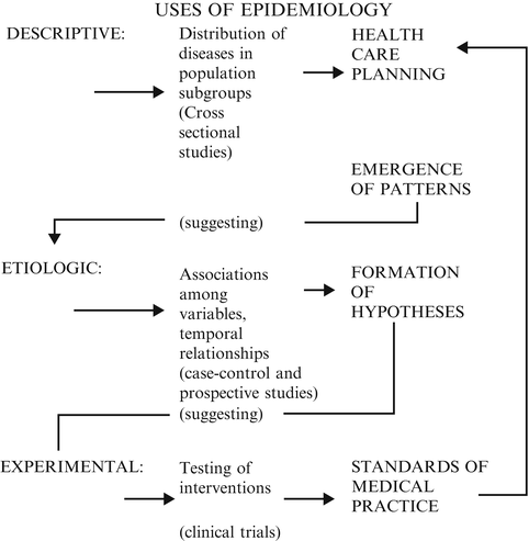
Figure 4.1
Uses of epidemiology
Descriptive epidemiology provides information on the pattern of diseases, on “who has what and how much of it,” information that is essential for health-care planning and rational allocation of resources. Such information may often uncover patterns of occurrence suggesting etiologic relationships and can lead to preventive strategies. Such studies are usually of the cross-sectional type and lead to the formation of hypotheses that can then be tested in case–control, prospective, and experimental studies. Clinical trials and other types of controlled studies serve to evaluate therapeutic modalities and other means of interventions and thus ultimately determine standards of medical practice, which in turn have impact on health-care planning decisions. In the following section, we will consider selected epidemiologic concepts.
4.2 Some Epidemiologic Concepts: Mortality Rates
In 1900, the three major causes of death were influenza or pneumonia, tuberculosis, and gastroenteritis. Today, the three major causes of death are heart disease, cancer, and accidents; the fourth is strokes. Stroke deaths have decreased dramatically over the last few decades probably due to the improved control of hypertension, one of the primary risk factors for stroke. These changing patterns of mortality reflect changing environmental conditions, a shift from acute to chronic illness, and an aging population subject to degenerative diseases. We know this from an analysis of rates.
The comparison of defined rates among different subgroups of individuals may yield clues to the existence of a health problem and may lead to the specification of conditions under which this identified health problem is likely to appear and flourish.
In using rates, the following points must be remembered:
(1)
A rate is a proportion involving a numerator and a denominator.
(2)
Both the numerator and the denominator must be clearly defined so that you know to which group (denominator) your rate refers.
(3)
The numerator is contained in (is a subset of) the denominator. This is in contrast to a ratio where the numerator refers to a different group from the denominator.
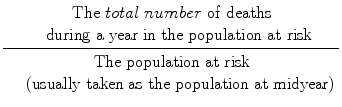
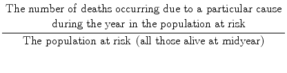
Mortality rates pertain to the number of deaths occurring in a particular population subgroup and often provide one of the first indications of a health problem. The following definitions are necessary before we continue our discussion:
The Crude Annual Mortality Rate (or death rate) is:
The Cause–Specific Annual Mortality Rate is:
The Age–Specific Annual Mortality Rate is:
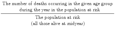
A reason for taking the population at midyear as the denominator is that a population may grow or shrink during the year in question and the midyear population is an estimate of the average number during the year. One can, however, speak of death rates over a 5-year period rather than a 1-year period, and one can define the population at risk as all those alive at the beginning of the period.
4.3 Age-Adjusted Rates
When comparing death rates between two populations, the age composition of the populations must be taken into account. Since older people have a higher number of deaths per 1,000 people, if a population is heavily weighted by older people, the crude mortality rate would be higher than in a younger population, and a comparison between the two groups might just reflect the age discrepancy rather than an intrinsic difference in mortality experience. One way to deal with this problem is to compare age-specific death rates, death rates specific to a particular age group. Another way that is useful when an overall summary figure is required is to use age-adjusted rates. These are rates adjusted to what they would be if the two populations being compared had the same age distributions as some arbitrarily selected standard population.
For example, the table below shows the crude and age-adjusted mortality rates for the United States at five time periods 15.7. The adjustment is made to the age distribution of the population in 1940 as well as the age distribution of the population in 2000. Thus, we see that in 1991, the age-adjusted rate was 5.1/1,000 when adjusted to 1940 standard, but the crude mortality rate was 8.6/1,000. This means that if in 1991 the age distribution of the population were the same as it was in 1940, then the death rate would have been only 5.1/1,000 people. The crude and age-adjusted rates for 1940 are the same because the 1940 population serves as the “standard” population whose age distribution is used as the basis for adjustment.
When adjusted to the year 2000 standard, the age-adjusted rate was 9.3. If in 1991 the age distribution were the same as in 2000, then the death rate would have been 9.3/1,000 people. So, age-adjusted rates depend on the standard population being used for the adjustment. Note that the age-adjusted rate based on the population in year 2000 is higher than the age-adjusted rate based on the population in 1940; this is because the population is older in year 2000.
Year | Crude mortality rate per 1,000 people | Age-adjusted rate (to population in 1940) | Age-adjusted rate (to population in 2000) |
|---|---|---|---|
1940 | 10.8 | 10.8 | 17.9 |
1960 | 9.5 | 7.6 | 13.4 |
1980 | 8.8 | 5.9 | 10.4 |
1991 | 8.6 | 5.1 | 9.3 |
2001 | 8.5 | Not computed after 1998 | 8.6 |
Although both crude and age-adjusted rates have decreased from 1940, the decrease in the age-adjusted rate is much greater. The percent change in crude mortality between 1940 and 1991 was (10.8–8.6)/10.8 = 20.4 %, whereas the percent change in the age-adjusted rate was (10.8–5.1)/10.8 = .528 or 52.8 %.
The reason for this is that the population is growing older. For instance, the proportion of persons 65 years and over doubled between 1920 and 1960, rising from 4.8 % of the population in 1920 to 9.6 % in 1969. After 1998, the National Center for Health Statistics used the population in 2000 as the standard population against which adjustments were made. The crude rate and the age-adjusted death rate in the year 2001 are similar, and that is because the age distribution in 2001 is similar to the age distribution in 2000 so age adjustment doesn’t really change the mortality rate much.
The age-adjusted rates are fictitious numbers—they do not tell you how many people actually died per 1,000, but how many would have died if the age compositions were the same in the two populations. However, they are appropriate for comparison purposes. Methods to perform age adjustment are described in Appendix 5.
4.4 Incidence and Prevalence
Prevalence and incidence are two measures of morbidity (illness).
Prevalence of a disease is defined as:

(This is also known as point prevalence, but more generally referred to just as “prevalence.”) For example, the prevalence of hypertension in 1973 among black males, ages 30–69, defined as a diastolic blood pressure (DBP) of 95 mmHg or more at a blood pressure screening program conducted by the Hypertension Detection and Follow-Up Program (HDFP),16 was calculated to be
![$$ \frac{4,268\kern0.5em with\kern0.5em DBP>95\; mmHg}{15,190\kern0.5em black\kern0.5em men\kern0.5em aged\kern0.5em 30-69\kern0.5em screened}\kern0.15em \times \kern0.15em 100=\kern0.15em 28.1\kern0.15em \mathrm{per}\kern0.15em 100\kern5em $$
” src=”/wp-content/uploads/2016/11/A270404_4_En_4_Chapter_Equma.gif”></DIV></DIV></DIV></DIV><br />
<DIV id=Par24 class=Para>Several points are to be noted about this definition:<br />
<DIV class=OrderedList><br />
<DIV class=ListItem><SPAN class=ItemNumber>(1)</SPAN><br />
<DIV class=ItemContent><br />
<DIV id=Par25 class=Para>The risk group (denominator) is clearly defined as black men, ages 30–69.</DIV></DIV><br />
<DIV class=ClearBoth> </DIV></DIV><br />
<DIV class=ListItem><SPAN class=ItemNumber>(2)</SPAN><br />
<DIV class=ItemContent><br />
<DIV id=Par26 class=Para>The point in time is specified as time of screening.</DIV></DIV><br />
<DIV class=ClearBoth> </DIV></DIV><br />
<DIV class=ListItem><SPAN class=ItemNumber>(3)</SPAN><br />
<DIV class=ItemContent><br />
<DIV id=Par27 class=Para>The definition of the disease is clearly specified as a diastolic blood pressure of 95 mmHg or greater. (This may include people who are treated for the disease but whose pressure is still high and those who are untreated.)</DIV></DIV><br />
<DIV class=ClearBoth> </DIV></DIV><br />
<DIV class=ListItem><SPAN class=ItemNumber>(4)</SPAN><br />
<DIV class=ItemContent><br />
<DIV id=Par28 class=Para>The numerator is the subset of individuals in the reference group (denominator) who satisfy the definition of the disease.</DIV></DIV><br />
<DIV class=ClearBoth> </DIV></DIV></DIV></DIV><br />
<DIV id=Par29 class=Para>Prevalence can also be age-adjusted to a standard population, meaning that the prevalence estimates are adjusted to what they would be if the population of interest had the same age distribution as some standard population (see Appendix 5 and Section <SPAN class=InternalRef><A href=]() 4.3). The prevalence of hypertension estimated by the Hispanic Community Health Study/Study of Latinos (HCHS/SOL),17 in 2007–2011, was found to be 25.5 % when age adjusted to the year 2000 standard. Hypertension was defined as systolic blood pressure of 140 mmHg or above or diastolic blood pressure of 90 mmHg or above, or on medications for high blood pressure.
4.3). The prevalence of hypertension estimated by the Hispanic Community Health Study/Study of Latinos (HCHS/SOL),17 in 2007–2011, was found to be 25.5 % when age adjusted to the year 2000 standard. Hypertension was defined as systolic blood pressure of 140 mmHg or above or diastolic blood pressure of 90 mmHg or above, or on medications for high blood pressure.


Incidence is defined as:
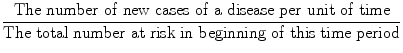
For example, studies have found that the 10-year incidence of a major coronary event (such as heart attack) among white men, ages 30–59, with diastolic blood pressure 105 mmHg or above at the time they were first seen, was found to be 183 per 1,000.18 This means that among 1,000 white men, ages 30–59, who had diastolic blood pressure above 105 mmHg at the beginning of the 10-year period of observation, 183 of them had a major coronary event (heart attack or sudden death) during the next 10 years. Among white men with diastolic blood pressure of <75 mmHg, the 10-year incidence of a coronary event was found to be 55/1,000. Thus, comparison of these two incidence rates, 183/1,000 for those with high blood pressure versus 55/1,000 for those with low blood pressure, may lead to the inference that elevated blood pressure is a risk factor for coronary disease.
Often, one may hear the word “incidence” used when what is really meant is prevalence. You should beware of such incorrect usage. For example, you might hear or even read in a medical journal that the incidence of diabetes in 1973 was 42.6 per 1,000 individuals, ages 45–64, when what is really meant is that the prevalence was 42.6/1,000. The thing to remember is that prevalence refers to the existence of a disease at a specific period in time, whereas incidence refers to new cases of a disease developing within a specified period of time.
Note that mortality rate is incidence, whereas morbidity may be expressed as incidence or prevalence. In a chronic disease, the prevalence is greater than the incidence because prevalence includes both new cases and existing cases that may have first occurred a long time ago, but the afflicted patients continued to live with the condition. For a disease that is either rapidly fatal or quickly cured, incidence and prevalence may be similar. Prevalence can be established by doing a survey or a screening of a target population and counting the cases of disease existing at the time of the survey. This is a cross-sectional study. Incidence figures are harder to obtain than prevalence figures since to ascertain incidence, one must identify a group of people free of the disease in question (i.e., a cohort), observe them over a period of time, and determine how many develop the disease over that time period. The implementation of such a process is difficult and costly.
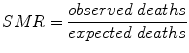
4.5 Standardized Mortality Ratio
The standardized mortality ratio (SMR) is the ratio of the number of deaths observed to the number of deaths expected. The number expected for a particular age group, for instance, is often obtained from population statistics.
4.6 Person-Years of Observation
Occasionally, one sees a rate presented as some number of events per person-years of observation, rather than per number of individuals observed during a specified period of time. Per person-years (or months) is useful as a unit of measurement when people are observed for different lengths of time. Suppose you are observing cohorts of people free of heart disease to determine whether the incidence of heart disease is greater for smokers than for those who quit. Quitters need to be defined, for example, as those who quit more than 5 years prior to the start of observation. One could define quitters differently and get different results, so it is important to specify the definition. Other considerations include controlling for the length of time smoked, which would be a function of age at the start of smoking and age at the start of the observation period, the number of cigarettes smoked, and so forth. But for simplicity, we will assume everyone among the smokers has smoked an equal amount and everyone among the quitters has smoked an equal amount prior to quitting.
We can express the incidence rate of heart disease per some unit of time, say 10 years, as the number who developed the disease during that time, divided by the number of people we observed (number at risk). However, suppose we didn’t observe everyone for the same length of time. This could occur because some people moved or died of other causes or were enrolled in the study at different times or for other reasons. In such a case, we could use as our denominator the number of person-years of observation.
For example, if individual 1 was enrolled at time 0 and was observed for 4 years, then lost to follow-up, he/she would have contributed 4 person-years of observation. Ten such individuals would contribute 40 person-years of observation. Another individual observed for 8 years would have contributed 8 person-years of observation, and 10 such individuals would contribute 80 person-years of observation for a total of 120 person-years. If six cases of heart disease developed among those observed, the rate would be 6 per 120 person-years, rather than 6/10 individuals observed. Note that if the denominator is given as person-years, you don’t know if it pertains to 120 people each observed for one year, or 12 people each observed for 10 years or some combination. Another problem with this method of expressing rates is that it reflects the average experience over the time span, but it may be that the rate of heart disease is the same for smokers as for quitters within the first 3 years and the rates begin to separate after that. In any case, various statistical methods are available for use with person-year analysis.
4.7 Dependent and Independent Variables
In research studies, we want to quantify the relationship between one set of variables, which we may think of as predictors or determinants, and some outcome or criterion variable in which we are interested. This outcome variable, which it is our objective to explain, is the dependent variable.
A dependent variable is a factor whose value depends on the level of another factor, which is termed an independent variable. In the example of cigarette smoking and lung cancer mortality, the duration and number of cigarettes smoked are independent variables upon which the lung cancer mortality depends (thus, lung cancer mortality is the dependent variable).
4.8 Types of Studies
In Section 1.4, we described different kinds of study designs, in the context of our discussion of the scientific method and of how we know what we know. These were observational studies, which may be cross-sectional, case–control, or prospective and experimental studies, which are clinical trials. In the following sections, we will consider the types of inferences that can be derived from data obtained from these different designs.
The objective is to assess the relationship between some factor of interest (the independent variable), which we will sometimes call exposure, and an outcome variable (the dependent variable).
The observational studies are distinguished by the point in time when measurements are made on the dependent and independent variables, as illustrated below. In cross-sectional studies, both the dependent and independent (outcome and exposure) variables are measured at the same time, in the present. In case–control studies, the outcome is measured now and exposure is estimated from the past. In prospective studies, exposure (the independent variable) is measured now and the outcome is measured in the future. In the next section, we will discuss the different inferences to be made from cross-sectional versus prospective studies.
Time of measurement | |||
|---|---|---|---|
Past | Present | Future | |
Cross-sectional | Exposure Outcome | ||
Case–control | Exposure | Outcome | |
Prospective | Exposure | Outcome | |
4.9 Cross-Sectional Versus Longitudinal Looks at Data
Prospective studies are sometimes also known as longitudinal studies, since people are followed longitudinally, over time. Examination of longitudinal data may lead to quite different inferences than those to be obtained from cross-sectional looks at data. For example, consider age and blood pressure.
Cross-sectional studies have repeatedly shown that the average systolic blood pressure is higher in each successive 10-year age group, while diastolic pressure increases for age groups up to age 50 and then reaches a plateau. One cannot, from these types of studies, say that blood pressure rises with age because the pressures measured for 30-year-old men, for example, were not obtained on the same individuals 10 years later when they were 40, but were obtained for a different set of 40-year-olds. To determine the effect of age on blood pressure, we would need to take a longitudinal or prospective look at the same individuals as they get older. One interpretation of the curve observed for diastolic blood pressure, for instance, might be that individuals over 60 who had very high diastolic pressures died off, leaving only those individuals with lower pressure alive long enough to be included in the sample of those having their blood pressure measured in the cross-sectional look.
The diagrams in Figure 4.2 illustrate the possible impact of a “cohort effect,” a cross-sectional view and a longitudinal view of the same data. (Letters indicate groups of individuals examined in a particular year.)
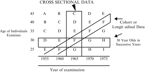
Figure 4.2
If you take the blood pressure of all groups in 1965 and compare group F to group D, you will have a cross-sectional comparison of 30-year-olds with 40-year-olds at a given point in time. If you compare group F in 1965 with group F (same individuals) in 1975, you will have a longitudinal comparison. If you compare group F in 1965 with group H in 1975, you will have a comparison of blood pressures of 30-year-olds at different points in time (a horizontal look).
These comparisons can lead to quite different conclusions, as is shown by the schematic examples in Figure 4.3 using fictitious numbers to represent average diastolic blood pressure.
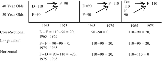
Figure 4.3
Cross-sectional versus longitudinal comparisons
In example (1), measurements in 1965 indicate that average diastolic blood pressure for 30-year-olds (group F) was 90 mmHg and for 40-year-olds (group D) it was 110 mmHg. Looking at group F 10 years later, when they were 40-year-olds, indicates their mean diastolic blood pressure was 90 mmHg. The following calculations result:
Cross-sectional look | D − F = 110 − 90 = 20 1965 1965 |
Conclusion | 40-year-olds have higher blood pressure than 30-year-olds (by 20 mmHg) |
Longitudinal look | F − F = 90 − 90 = 0 1975 1965 |
Conclusion | Blood pressure does not rise with age |
Horizontal look (cohort comparisons) | F − F = 90 − 110 = −20 1975 1965 |
Conclusion | 40-year-olds in 1975 have lower blood pressure than 40-year-olds did in 1965 |
A possible interpretation: Blood pressure does not rise with age, but different environmental forces were operating for the F cohort than for the D cohort.
In example (2), we have
Cross-sectional look | D − F = 90 − 90 = 0 mmHg 1965 1965 |
Conclusion | From cross-sectional data, we conclude that blood pressure is not higher with older age |
Longitudinal look | F − F = 110 − 90 = 20 1975 1965 |
Conclusion | From longitudinal data, we conclude that blood pressure goes up with age |
Horizontal look | F − D = 110 − 90 = 20 1975 196 |
Conclusion | 40-year-olds in 1975 have higher blood pressure than 40-year-olds in 1965 |
A possible interpretation: Blood pressure does rise with age and different environmental factors operated on the F cohort than on the D cohort.
In example (3), we have
Cross-sectional look | D − F = 110 − 90 = 20 1965 1965 |
Conclusion | Cross-sectionally, there was an increase in blood pressure for 40-year-olds over that for 30-year-olds |
Longitudinal look | F − F = 110 − 90 = 20 1975 1965 |
Conclusion | Longitudinally, it is seen that blood pressure increases with increasing age |
Horizontal look | F − D = 110 − 110 = 0 1975 1965 |
Conclusion | There was no change in blood pressure among 40-year-olds over the 10 year period |
A possible interpretation: Blood pressure does go up with age (supported by both longitudinal and cross-sectional data), and environmental factors affect both cohorts similarly.
4.10 Measures of Relative Risk: Inferences from Prospective Studies (the Framingham Study)
In epidemiologic studies, we are often interested in knowing how much more likely an individual is to develop a disease if he or she is exposed to a particular factor than the individual who is not so exposed. A simple measure of such likelihood is called relative risk (RR). It is the ratio of two incidence estimates: the rate of development of the disease for people with the exposure factor, divided by the rate of development of the disease for people without the exposure factor. Suppose we wish to determine the effect of high blood pressure (hypertension) on the development of cardiovascular disease (CVD). To obtain the relative risk, we need to calculate the incidence rates. We can use the data from a classic prospective study, the Framingham Heart Study.19
This was a pioneering prospective epidemiologic study of a population sample in the small town of Framingham, Massachusetts. Beginning in 1948, a cohort of people was selected to be followed up biennially. The term cohort refers to a group of individuals followed longitudinally over a period of time. A birth cohort, for example, would be the population of individuals born in a given year. The Framingham cohort was a sample of people chosen at the beginning of the study period and included men and women aged 30–62 years at the start of the study. These individuals were observed over a 20-year period, and morbidity and mortality associated with cardiovascular disease were determined. A standardized hospital record and death certificate were obtained, clinic examination was repeated at 2-year intervals, and the major concern of the Framingham study has been to evaluate the relationship of characteristics determined in well persons to the subsequent development of disease.
Through this study, “risk factors” for cardiovascular disease were identified. The risk factors are antecedent physiologic characteristics or dietary and living habits, whose presence increases the individual’s probability of developing cardiovascular disease at some future time. Among the most important predictive factors identified in the Framingham study were elevated blood pressure, elevated serum cholesterol, and cigarette smoking. Elevated blood glucose and abnormal resting electrocardiogram findings are also predictive of future cardiovascular disease.
Relative risk can be determined by the following calculation:

From the Framingham data, we calculate for men in the study the


This means that a man with definite hypertension is 2.85 times more likely to develop CVD in an 18-year period than a man who does not have hypertension. For women, the relative risk is

This means that hypertension carries a somewhat greater relative risk for women. But note that the absolute risk for persons with definite hypertension (i.e., the incidence of CVD) is greater for men than for women, being 353.2 per 10,000 men versus 187.9 per 10,000 women.
The incidence estimates given above have been age adjusted. Age adjustment is discussed in Section 4.3. Often, one may want to adjust for other variables such as smoking status, diabetes, cholesterol levels, and other factors that may also be related to outcome. This may be accomplished by multiple logistic regression analysis and by Cox proportional hazards analysis, which are described in Sections. 4.17 and 4.19, respectively, but first we will describe how relative risk can be calculated from prospective studies or estimated from case–control studies.
4.11 Calculation of Relative Risk from Prospective Studies
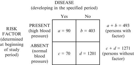
Relative risk can be determined directly from prospective studies by constructing a 2 × 2 table as follows20:
Relative risk is
 Relative risk, or hazard ratio, can be calculated from Cox proportional hazards regression models (which allow for adjustment for other variables) as described in Section 4.19.
Stay updated, free articles. Join our Telegram channel
Full access? Get Clinical Tree
